17 Squared multiple correlation and variance decomposition in linear regression

In this chapter we first introduce the (squared) multiple correlation and the multiple and adjusted \(R^2\) coefficients as estimators. Subsequently we discuss variance decomposition.

17.1 Squared multiple correlation \(\Omega^2\) and the \(R^2\) coefficient

In the previous chapter we encountered the following quantity: \[ \Omega^2 = \boldsymbol P_{y \boldsymbol x} \boldsymbol P_{\boldsymbol x\boldsymbol x}^{-1} \boldsymbol P_{\boldsymbol xy} = \sigma_y^{-2} \boldsymbol \Sigma_{y \boldsymbol x} \boldsymbol \Sigma_{\boldsymbol x\boldsymbol x}^{-1} \boldsymbol \Sigma_{\boldsymbol xy} \]

With \(\boldsymbol \beta=\boldsymbol \Sigma_{\boldsymbol x\boldsymbol x}^{-1} \boldsymbol \Sigma_{\boldsymbol xy}\) and \(\beta_0=\mu_y- \boldsymbol \beta^T \boldsymbol \mu_{\boldsymbol x}\) it is straightforward to verify the following:

• the cross-covariance between \(y\) and \(y^{\star}\) is \[ \begin{split} \text{Cov}(y, y^{\star}) &= \boldsymbol \Sigma_{y \boldsymbol x} \boldsymbol \beta= \boldsymbol \Sigma_{y \boldsymbol x} \boldsymbol \Sigma_{\boldsymbol x\boldsymbol x}^{-1} \boldsymbol \Sigma_{\boldsymbol xy} \\ & = \sigma^2_y \boldsymbol P_{y \boldsymbol x} \boldsymbol P_{\boldsymbol x\boldsymbol x}^{-1} \boldsymbol P_{\boldsymbol xy} = \sigma_y^2 \Omega^2\\ \end{split} \]
• the (signal) variance of \(y^{\star}\) is \[ \begin{split} \text{Var}(y^{\star}) &= \boldsymbol \beta^T \boldsymbol \Sigma_{\boldsymbol x\boldsymbol x} \boldsymbol \beta= \boldsymbol \Sigma_{y \boldsymbol x} \boldsymbol \Sigma_{\boldsymbol x\boldsymbol x}^{-1} \boldsymbol \Sigma_{\boldsymbol xy} \\ & = \sigma^2_y \boldsymbol P_{y \boldsymbol x} \boldsymbol P_{\boldsymbol x\boldsymbol x}^{-1} \boldsymbol P_{\boldsymbol xy} = \sigma_y^2 \Omega^2\\ \end{split} \]

hence the correlation \(\text{Cor}(y, y^{\star}) = \frac{\text{Cov}(y, y^{\star})}{\text{SD}(y) \text{SD}(y^{\star})} = \Omega\) with \(\Omega \geq 0\).

This helps to understand the \(\Omega\) and \(\Omega^2\) coefficients:

• \(\Omega\) is the linear correlation between the response (\(y\)) and prediction \(y^{\star}\).

• \(\Omega^2\) is called the squared multiple correlation between the scalar \(y\) and the vector \(\boldsymbol x\).

• Note that if we only have one predictor (if \(x\) is a scalar) then \(\boldsymbol P_{x x} = 1\) and \(\boldsymbol P_{y x} = \rho_{yx}\) so the multiple squared correlation coefficient reduces to squared correlation \(\Omega^2 = \rho_{yx}^2\) between two scalar random variables \(y\) and \(x\).

17.1.1 Estimation of \(\Omega^2\) and the multiple \(R^2\) coefficient

The multiple squared correlation coefficient \(\Omega^2\) can be estimated by plug-in of empirical estimates for the corresponding correlation matrices: \[R^2 = \hat{\boldsymbol P}_{y \boldsymbol x} \hat{\boldsymbol P}_{\boldsymbol x\boldsymbol x}^{-1} \hat{\boldsymbol P}_{\boldsymbol xy} = \hat{\sigma}_y^{-2} \hat {\boldsymbol \Sigma}_{y \boldsymbol x} \hat{\boldsymbol \Sigma}_{\boldsymbol x\boldsymbol x}^{-1} \hat{\boldsymbol \Sigma}_{\boldsymbol xy}\] This estimator of \(\Omega^2\) is called the multiple \(R^2\) coefficient.

If the same scale factor \(1/n\) or \(1/(n-1)\) is used in estimating the variance \(\sigma^2_y\) and the covariances \(\boldsymbol \Sigma_{\boldsymbol x\boldsymbol x}\) and \(\boldsymbol \Sigma_{y \boldsymbol x}\) then this factor will cancel out.

Above we have seen that \(\Omega^2\) is directly linked with the noise variance via \[ \text{Var}(\varepsilon) =\sigma^2_y (1-\Omega^2) \,. \] so we can express the squared multiple correlation as \[ \Omega^2 = 1- \text{Var}(\varepsilon) / \sigma^2_y \]

The maximum likelihood estimate of the noise variance \(\text{Var}(\varepsilon)\) (also called residual variance) can be computed from the residual sum of squares \(RSS = \sum_{i=1}^n (y_i -\hat{y}_i)^2\) as follows: \[ \widehat{\text{Var}}(\varepsilon)_{ML} = \frac{RSS}{n} \] whereas the unbiased estimate is obtained by \[ \widehat{\text{Var}}(\varepsilon)_{UB} = \frac{RSS}{n-d-1} = \frac{RSS}{df} \] where the degree of freedom is \(df=n-d-1\) and \(d\) is the number of predictors.

Similarly, we can find the maximum likelihood estimate \(v_y^{ML}\) for \(\sigma^2_y\) (with factor \(1/n\)) as well as an unbiased estimate \(v_y^{UB}\) (with scale factor \(1/(n-1)\))

The multiple \(R^2\) coefficient can then be written as \[ R^2 =1- \widehat{\text{Var}}(\varepsilon)_{ML} / v_y^{ML} \] Note we use MLEs.

In contrast, the so-called adjusted multiple \(R^2\) coefficient is given by \[ R^2_{\text{adj}}=1- \widehat{\text{Var}}(\varepsilon)_{UB} / v_y^{UB} \] where the unbiased variances are used.

Both \(R^2\) and \(R^2_{\text{adj}}\) are estimates of \(\Omega^2\) and are related by \[ 1-R^2 = (1- R^2_{\text{adj}}) \, \frac{df}{n-1} \]

17.1.2 R commands

In R the command lm() fits the linear regression model.

In addition to the regression cofficients (and derived quantities) the R function lm() also lists

• the multiple R-squared \(R^2\),
• the adjusted R-squared \(R^2_{\text{adj}}\),
• the degrees of freedom \(df\) and
• the residual standard error \(\sqrt{\widehat{\text{Var}}(\varepsilon)_{UB}}\) (computed from the unbiased variance estimate).

See also Worksheet R3 which provides R code to reproduce the exact output of the native lm() R function.

17.2 Variance decomposition in regression

The squared multiple correlation coefficient is useful also because it plays an important role in the decomposition of the total variance:

• total variance: \(\text{Var}(y) = \sigma^2_y\)
• unexplained variance (irreducible error): \(\sigma^2_y (1-\Omega^2) = \text{Var}(\varepsilon)\)
• the explained variance is the complement: \(\sigma^2_y \Omega^2 = \text{Var}(y^{\star})\)

In summary:

\[\text{Var}(y) = \text{Var}(y^{\star}) + \text{Var}(\varepsilon)\] becomes \[\underbrace{\sigma^2_y}_{\text{total variance}} = \underbrace{\sigma_y^2 \Omega^2}_{\text{explained variance}} + \underbrace{ \sigma^2_y (1-\Omega^2)}_{\text{unexplained variance}}\]

The unexplained variance measures the fit after introducing predictors into the model (smaller means better fit). The total variance measures the fit of the model without any predictors. The explained variance is the difference between total and unexplained variance, it indicates the increase in model fit due to the predictors.

17.2.1 Law of total variance and variance decomposition

The law of total variance is

\[\underbrace{\text{Var}(y)}_{\text{total variance}} = \underbrace{\text{Var}( \text{E}(y | \boldsymbol x) ) }_{\text{explained variance}} + \underbrace{ \text{E}( \text{Var}( y | \boldsymbol x) )}_{\text{unexplained variance}}\]

provides a very general decomposition in explained and unexplained parts of the variance that is valid regardless of the form of the distributions \(F_{y, \boldsymbol x}\) and \(F_{y | \boldsymbol x}\).

In regression it conncects variance decomposition and conditioning. If you plug-in the conditional expections for the multivariate normal model (cf. previous chapter) we recover

\[\underbrace{\sigma^2_y}_{\text{total variance}} = \underbrace{\sigma_y^2 \Omega^2 }_{\text{explained variance}} + \underbrace{ \sigma^2_y (1-\Omega^2)}_{\text{unexplained variance}}\]

17.2.2 Related quantities

Using the above three quantities (total variance, explained variance, and unexplained variance) we can construct a number of scores:

1. coefficient of determination, squared multiple correlation:

\[ \frac{\text{explained var}}{\text{total var}} = \frac{\sigma_y^2 \Omega^2}{\sigma_y^2} = \Omega^2 \] (range 0 to 1, with 1 indicating perfect fit)

2. coefficient of non-determination, coefficient of alienation:

\[ \frac{\text{unexplained var}}{\text{total var}} = \frac{\sigma_y^2 (1-\Omega^2)}{\sigma_y^2} = 1-\Omega^2 \] (range 0 to 1, with 0 indicating perfect fit)

3. \(F\) score, \(t^2\) score:

\[ \frac{\text{explained var}}{\text{unexplained var}} = \frac{\sigma_y^2 \Omega^2}{\sigma_y^2 (1-\Omega^2)} = \frac{\Omega^2}{1-\Omega^2} = \mathcal{F} = \frac{\tau^2}{n} \] (range 0 to \(\infty\), with \(\infty\) indicating perfect fit)

Note that the \(\mathcal{F}\) and \(\tau^2\) scores are population versions of the \(F\) and \(t^2\) statistics.

Also note that \(\Omega^2 = \frac{\tau^2}{\tau^2 + n} = \frac{\mathcal{F}}{\mathcal{F} + 1}\) links squared correlation with squared \(t\)-scores and \(F\)-scores.

17.3 Sample version of variance decomposition

If \(\Omega^2\) and \(\sigma^2_y\) are replaced by their MLEs this can be written in a sample version as follows using data points \(y_i\), predictions \(\hat{y}_i\) and \(\bar{y} = \frac{1}{n}\sum_{i=1}^n {y_i}\)

\[\underbrace{\sum_{i=1}^n (y_i-\bar{y})^2}_{\text{total sum of squares (TSS)}} = \underbrace{\sum_{i=1}^n (\hat{y}_i-\bar{y})^2 }_{\text{explained sum of squares (ESS)}} + \underbrace{\sum_{i=1}^n (y_i-\hat{y}_i)^2 }_{\text{residual sum of squares (RSS)}}\]

Note that TSS, ESS and RSS all scale with \(n\). Using data vector notation the sample-based variance decomposition can be written in form of the Pythagorean theorem: \[\underbrace{|| \boldsymbol y-\bar{y} \boldsymbol 1\ ||^2}_{\text{total sum of squares (TSS)}} = \underbrace{||\hat{\boldsymbol y}-\bar{y} \boldsymbol 1||^2 }_{\text{explained sum of squares (ESS)}} + \underbrace{|| \boldsymbol y-\hat{\boldsymbol y} ||^2 }_{\text{residual sum of squares (RSS)}}\]

17.3.1 Geometric interpretation of regression as orthogonal projection:

The above equation can be further simplified to

\[|| \boldsymbol y||^2 = ||\hat{\boldsymbol y}||^2 + \underbrace{|| \boldsymbol y-\hat{\boldsymbol y} ||^2 }_{\text{RSS}} \]

Geometrically speaking, this implies \(\hat{\boldsymbol y}\) is an orthogonal projection of \(\boldsymbol y\), since the residuals \(\boldsymbol y-\hat{\boldsymbol y}\) and the predictions \(\hat{\boldsymbol y}\) are orthogonal (by construction!).

This also valid for the centered versions of the vectors, i.e. \(\hat{\boldsymbol y}-\bar{y} \boldsymbol 1_n\) is an orthogonal projection of \(\boldsymbol y-\bar{y} \boldsymbol 1_n\) (see Figure).

Also note that the angle \(\theta\) between the two centered vectors is directly related to the (estimated) multiple correlation, with \(R = \cos(\theta) = \frac{||\hat{\boldsymbol y}-\bar{y} \boldsymbol 1_n ||}{|| \boldsymbol y-\bar{y} \boldsymbol 1_n||}\), or \(R^2 = \cos(\theta)^2 = \frac{||\hat{\boldsymbol y}-\bar{y} \boldsymbol 1_n ||^2}{|| \boldsymbol y-\bar{y} \boldsymbol 1_n||^2} = \frac{\text{ESS}}{\text{TSS}}\).

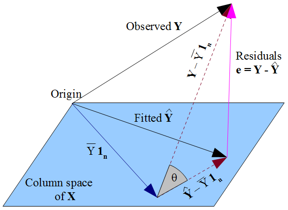
Source of Figure: Stack Exchange