18 Prediction and variable selection

In this chapter we discuss how to compute (lower bounds) of the prediction error and how to select variables relevant for prediction

18.1 Prediction and prediction intervals

Learning the regression function from (training) data is only the first step in application of regression models.

The next step is to actually make prediction of future outcomes \(y^{\text{test}}\) given test data \(\boldsymbol x^{\text{test}}\): \[ y^{\text{test}} = \hat{y}(\boldsymbol x^{\text{test}}) = \hat{f}_{\hat{\beta}_0, \hat{\boldsymbol \beta}}(\boldsymbol x^{\text{test}}) \]

Note that \(y^{\text{test}}\) is a point estimator. Is it possible also to construct a corresponding interval estimate?

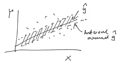
The answer is yes, and leads back to the conditioning approach:

\[y^\star = \text{E}(y| \boldsymbol x) = \beta_0 + \boldsymbol \beta^T \boldsymbol x\]

\[\text{Var}(\varepsilon) = \text{Var}(y|\boldsymbol x) = \sigma^2_y (1-\Omega^2)\]

We know that the mean squared prediction error for \(y^{\star}\) is \(\text{E}((y -y^{\star})^2)=\text{Var}(\varepsilon)\) and that this is the minimal irreducible error. Hence, we may use \(\text{Var}(\varepsilon)\) as the minimum variability for the prediction.

The corresponding prediction interval is \[\left[ y^{\star}(\boldsymbol x^{\text{test}}) \pm c \times \text{SD}(\varepsilon) \right]\] where \(c\) is some suitable constant (e.g. 1.96 for symmetric 95% normal intervals).

However, please note that the prediction interval constructed in this fashion will be an underestimate. The reason is that this assumes that we employ \(y^{\star} = \beta_0 + \boldsymbol \beta^T \boldsymbol x\) but in reality we actually use \(\hat{y} = \hat{\beta}_0 + \hat{\boldsymbol \beta}^T \boldsymbol x\) for prediction — note the estimated coefficients! We recall from an earlier chapter (best linear predictor) that this leads to increase of MSPE compared with using the optimal \(\beta_0\) and \(\boldsymbol \beta\).

Thus, for better prediction intervals we would need to consider the mean squared prediction error of \(\hat{y}\) that can be written as \(\text{E}((y -\hat{y})^2) = \text{Var}(\varepsilon) + \delta\) where \(\delta\) is an additional error term due to using an estimated rather than the true regression function. \(\delta\) typically declines with \(1/n\) but can be substantial for small \(n\) (in particular as it usually depends on the number of predictors \(d\)).

For more details on this we refer to later modules on regression.

18.2 Variable importance and prediction

Another key question in regression modelling is to find out predictor variables \(x_1, x_2, \dots, x_d\) are actually important for predicting the outcome \(y\).

\(\rightarrow\) We need to study variable importance measures (VIM).

18.2.1 How to quantify variable importance?

A variable \(x_i\) is important if it improves prediction of the response \(y\).

Recall variance decomposition:

\[\text{Var}(y) = \sigma_y^2 = \underbrace{\sigma^2_y\Omega^2}_{\text{explained variance}} + \underbrace{\sigma^2_y(1-\Omega^2)}_{\text{unexplained/residual variance =} \text{Var}(\varepsilon)}\]

• \(\Omega^2\) squared multiple correlation \(\in [0,1]\)
• \(\Omega^2\) large \(\rightarrow 1\) predictor variables explain most of \(\sigma_y^2\)
• \(\Omega^2\) small \(\rightarrow 0\) linear model fails and predictors do not explain variability
• \(\Rightarrow\) If a predictor helps to \(\begin{array}{ll} \text{increase explained variance} \\ \text{decrease unexplained variance} \end{array}\) then it is important!
• \(\Omega^2 = \boldsymbol P_{y\boldsymbol x} \boldsymbol P_{\boldsymbol x\boldsymbol x}^{-1} \boldsymbol P_{\boldsymbol xy} \hat{=}\) a function of the \(X\)!

VIM: which predictors contribute most to \(\Omega^2\)

18.2.2 Some candidates for VIMs

1. The regression coefficients \(\boldsymbol \beta\)

   • \(\boldsymbol \beta= \boldsymbol \Sigma^{-1}_{\boldsymbol x\boldsymbol x} \boldsymbol \Sigma_{\boldsymbol xy}= \boldsymbol V_{\boldsymbol x}^{-1/2} \boldsymbol P_{\boldsymbol x\boldsymbol x}^{-1} \boldsymbol P_{\boldsymbol xy} \sigma_y\)
   • Not a good VIM since \(\boldsymbol \beta\) contains the scale!
   • Large \(\hat{\beta}_i\) does not indicate that \(x_i\) is important.
   • Small \(\hat{\beta}_i\) does not indicate that \(x_i\) is not important.

2. Standardised regression coefficients \(\boldsymbol \beta_{\text{std}}\)

   • \(\boldsymbol \beta_{\text{std}} = \boldsymbol P_{\boldsymbol x\boldsymbol x}^{-1} \boldsymbol P_{\boldsymbol xy}\)
   • implies \(\text{Var}(y)=1\), \(\text{Var}(x_i)=1\)
   • These do not contain the scale (so better than \(\hat{\beta}\))
   • But still unclear how this relates to decomposition of variance

3. Squared marginal correlations \(\rho_{y, x_i}^2\)

   Consider case of uncorrelated predictors: \(\boldsymbol P_{\boldsymbol x\boldsymbol x}=\boldsymbol I\) (no correlation among \(x_i\))

   \[\Rightarrow \Omega^2 = \boldsymbol P_{y\boldsymbol x} \boldsymbol P_{\boldsymbol xy} = \sum^d_{i=1} \rho_{y, x_i}^2\]

   \(\rho_{y, x_i}^2 = \text{Cor}(y, x_i)\) is the marginal correlation between \(y\) and \(x_i\), and \(\Omega^2\) is (for uncorrelated predictors) the sum of squared marginal correlations.

   • If \(\boldsymbol P_{\boldsymbol x\boldsymbol x}=\boldsymbol I\), then ranking predictors by \(\rho_{y, x_i}^2\) is optimal!
   • The predictor with largest marginal correlation reduces the unexplained variance most!
   • good news: even if there is weak correlation among predictors the marginal correlations are still good as VIM (but then they will not perfectly add up to \(\Omega^2\))
   • Advantage: very simple but often also very effective.
   • Caution! If there is strong correlation in \(\boldsymbol P_{\boldsymbol x\boldsymbol x}\), then there is colinearity (in this case it is oftern best to remove one of the strongly correlated variables, or to merge the correlated variables).

Often, ranking predictors by their squared marginal correlations is done as a prefiltering step (independence screening).

18.3 Regression \(t\)-scores.

18.3.1 Wald statistic for regression coefficients

So far, we discussed three obvious candidates for for variable importance measures (regression coefficients, standardised regression coefficients, marginal correlations).

In this section we consider a further quantity, the regression \(t-\)score:

Recall that ML estimation of the regression coefficients yields

• a point estimate \(\hat{\boldsymbol \beta}\)
• the (asymptotic) variance \(\widehat{\text{Var}}(\hat{\boldsymbol \beta})\)
• the asymptotic normal distribution \(\hat{\boldsymbol \beta} \overset{a}{\sim} N_d(\boldsymbol \beta, \widehat{\text{Var}}(\hat{\boldsymbol \beta}))\)

Corresponding to each predictor \(x_i\) we can construct from the above a \(t\)-score \[ t_i = \frac{\hat{\beta}_i}{\widehat{\text{SD}}(\hat{\beta}_i)} \] where the standard deviations are computed by \(\widehat{\text{SD}}(\hat{\beta}_i) = \text{Diag}(\widehat{\text{Var}}(\hat{\boldsymbol \beta}))_{i}\). This corresponds to the Wald statistic to test that the underlying true regression coefficient is zero (\(\beta_i =0\)).

Correspondingly, under the null hypthesis that \(\beta_i=0\) asymptotically for large \(n\) the regression \(t\)-score is standard normal distributed: \[ t_i \overset{a}{\sim} N(0,1) \] This allows to compute (symmetric) \(p\)-values \(p = 2 \Phi(-|t_i|)\) where \(\Phi\) is the standard normal distribution function.

For finite \(n\), assuming normality of the observation and using the unbiased estimate for variance when computing \(t_i\), the exact distribution of \(i_i\) is given by the Student-\(t\) distribution: \[ t_i \sim t_{n-d-1} \]

Regression \(t\)-scores can thus be used to test whether a regression coefficient is zero. A large magnitude of the \(t_i\) score indicates that the hypothesis \(\beta_i=0\) can be rejected. Thus, a small \(p\)-value (say smaller than 0.05) signals that the regression coefficient is non-zero and hence that the corresponding predictor variable should be included in the model.

This allows rank predictor variables by \(|t_i|\) or the corresponding \(p\)-values with regard to their relevance in the linear model. Typically, in order to simplify a model, predictors with the largest \(p\)-values (and thus smallest absolute \(t\)-scores) may be removed from a model. However, note that having a \(p\)-value say larger than 0.05 by itself is not sufficient to declare a regression coefficient to be zero (because in classical statistical testing you can only reject the null hypothesis, but not accept it!).

Note that by construction the regression \(t\)-scores do not depend on the scale, so when the original data are rescaled this will not affect the corresponding regression \(t\)-scores. Furthermore, if \(\widehat{\text{SD}}(\hat{\beta}_i)\) is small, then the regression \(t\)-score \(t_i\) can still be large even if \(\hat{\beta}_i\) is small!

18.3.2 Computing

When you perform regression analysis in R (or another statistical software package) the computer will return the following:

\[\begin{align*} \begin{array}{cc} \hat{\beta}_i\\ \text{Estimated}\\ \text{repression}\\ \text{coefficient}\\ \\ \end{array} \begin{array}{cc} \widehat{\text{SD}}(\hat{\beta}_i)\\ \text{Error of}\\ \hat{\beta}_i\\ \\ \\ \end{array} \begin{array}{cc} t_i = \frac{\hat{\beta}_i}{\widehat{\text{SD}}(\hat\beta_i)}\\ \text{t-score}\\ \text{computed from }\\ \text{first two columns}\\ \\ \end{array} \begin{array}{cc} \text{p-values}\\ \text{for } t_i\\ \text{based on t-distribution}\\ \\ \\ \end{array} \begin{array}{ll} \text{Indicator of}\\ \text{Significance}\\ \text{* } 0.9\\ \text{** } 0.95\\ \text{*** } 0.99\\ \end{array} \end{align*}\]

In the lm() function in R the standard deviation is the square root of the unbiased estimate of the variance (but note that it itself is not unbiased!).

18.3.3 Connection with partial correlation

The deeper reason why ranking predictors by regression \(t\)-scores and associated \(p\)-values is useful is their link with partial correlation.

In particular, the (squared) regression \(t\)-score can be 1:1 transformed into the (estimated) (squared) partial correlation \[ \hat{\rho}_{y, x_i | x_{j \neq i}}^2 = \frac{t_i^2}{t_i^2 + df} \] with \(df=n-d-1\), and it can be shown that the \(p\)-values for testing that \(\beta_i=0\) are exactly the same as the \(p\)-values for testing that the partial correlation \(\rho_{y, x_i | x_{j \neq i}}\) vanishes!

Therefore, ranking the predictors \(x_i\) by regression \(t\)-scores leads to exactly the same ranking and \(p\)-values as partial correlation!

18.3.4 Squared Wald statistic and the \(F\) statistic

In the above we looked at individual regression coefficients. However, we can also construct a Wald test using the complete vector \(\hat{\boldsymbol \beta}\). The squared Wald statistic to test that \(\boldsymbol \beta= 0\) is given by \[ \begin{split} t^2 & = \hat{\boldsymbol \beta}^T \widehat{\text{Var}}(\hat{\boldsymbol \beta}^{-1}) \hat{\boldsymbol \beta}\\ & = \left( \hat{\boldsymbol \Sigma}_{y \boldsymbol x} \hat{\boldsymbol \Sigma}_{\boldsymbol x\boldsymbol x}^{-1} \right) \left( \frac{n}{ \widehat{\sigma^2_{\varepsilon}} } \hat{\boldsymbol \Sigma}_{\boldsymbol x\boldsymbol x}\right) \left( \hat{\boldsymbol \Sigma}_{\boldsymbol x\boldsymbol x}^{-1} \hat{\boldsymbol \Sigma}_{\boldsymbol xy} \right) \\ & = \frac{n}{ \widehat{\sigma^2_{\varepsilon}} } \hat{\boldsymbol \Sigma}_{y \boldsymbol x} \hat{\boldsymbol \Sigma}_{\boldsymbol x\boldsymbol x}^{-1} \hat{\boldsymbol \Sigma}_{\boldsymbol xy} \\ & = \frac{n}{ \widehat{\sigma^2_{\varepsilon}} } \hat{\sigma}_y^{2} R^2\\ \end{split} \] With \(\widehat{\sigma^2_{\varepsilon}} / \hat{\sigma}_y^{2} = 1- R^2\) we finally get the related \(F\) statistic \[ \frac{t^2}{n} = \frac{R^2}{1-R^2} = F \] which is a function of \(R^2\). If \(R^2=0\) then \(F=0\). If \(R^2\) is large (\(< 1\)) then \(F\) is large as well (\(< \infty\)) and the null hypothesis \(\boldsymbol \beta= 0\) can be rejected, which implies that at least one regression coefficient is non-zero. Note that the squared Wald statistic \(t^2\) is asymptotically \(\chi^2_d\) distributed which is useful to find critical values and to compute \(p\)-values.

18.4 Further approaches for variable selection

In addition to ranking by marginal and partial correlation, there are many other approaches for variable selection in regression!

1. Search-based methods:

   • search through subsets of linear models for \(d\) variables, ranging from full model (including all predictors) to the empty model (includes no predictor) and everything inbetween.
   • Problem: exhaustive search not possible even for relatively small \(d\) as space of models is very large!
   • Therefore heuristic approaches such as forward selection (adding predictors), backward selection (removing predictors), or monte-carlo random search are employed.
   • Problem: maximum likelihood cannot be used for choosing among the models - since ML will always pick the best model. Therefore, penalised ML criteria such as AIC or Bayesian criteria are often employed instead.

2. Integrative estimation and variable selection:

   • there are methods that fit the regression model and perform variable selection simultaneously.
   • the most well-known approach of this type is “lasso” regression (Tibshirani 1996)
   • This applies a (generalised) linear model with ML plus L1 penalty.
   • Alternative: Bayesian variable selection and estimation procedures

3. Entropy-based variable selection:

   As seen above, two of the most popular approaches in linear models are based on correlation, either marginal correlation or partial correlation (via regression \(t\)-scores).

   Correlation measures can be generalised to non-linear settings. One very popular measure is the mutual information which is computed using the KL divergence. In case of two variables \(x\) and \(y\) with joint normal distribution and correlation \(\rho\) the mutual information is a function of the correlation: \[\text{MI}(x,y) = \frac{1}{2} \log (1-\rho^2)\]

   In regression he mutual information between the response \(y\) and predictor \(x_i\) is \(\text{MI}(y, x_i)\), and this widely used for feature selection, in particular in machine learning.

4. FDR based variable selection in regression:

   Feature selection controling the false discovery rate (FDR) among the selected features are becoming more popular, in particular a number of procedures using so-called “knockoffs”, see https://web.stanford.edu/group/candes/knockoffs/ .

5. Variable importance using Shapley values:

   Borrowing a concept from game theory Shapley values have recently become popular in machine learning to evaluate the variable importance of predictors in nonlinear models. Their relationship to other statistical methods for measuring variable importance is the focus of current research.