15 Linear Regression

15.1 The linear regression model

In this module we assume that \(f\) is a linear function: \[f(x_1, \ldots, x_d) = \beta_0 + \sum^{d}_{j=1} \beta_j x_j = y^{\star}\]

In vector notation: \[ f(\boldsymbol x) = \beta_0 + \boldsymbol \beta^T \boldsymbol x= y^{\star} \] with \(\boldsymbol \beta=\begin{pmatrix} \beta_1 \\ \vdots \\ \beta_d \end{pmatrix}\) and \(\boldsymbol x=\begin{pmatrix} x_1 \\ \vdots \\ x_d \end{pmatrix}\)

Therefore, the linear regression model is \[ \begin{split} y &= \beta_0 + \sum^{d}_{j=1} \beta_j x_j + \varepsilon\\ &= \beta_0 + \boldsymbol \beta^T \boldsymbol x+\varepsilon \\ &= y^{\star} +\varepsilon \end{split} \] where:

• \(\beta_0\) is the intercept
• \(\boldsymbol \beta= (\beta_1,\ldots,\beta_d)^T\) are the regression coefficients
• \(\boldsymbol x= (x_1,\ldots,x_d)^T\) is the predictor vector containing the predictor variables

15.2 Interpretation of regression coefficients and intercept

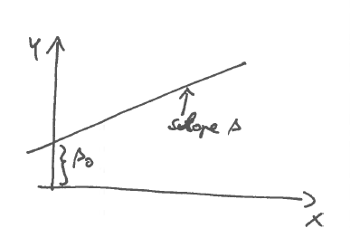
• The regression coefficient \(\beta_i\) corresponds to the slope (first partial derivative) of the regression function in the direction of \(x_i\). In other words, the gradient of \(f(\boldsymbol x)\) are the regression coefficients: \(\nabla f(\boldsymbol x) = \boldsymbol \beta\)
• The intercept \(\beta_0\) is the offset at the origin (\(x_1=x_2=\ldots=x_d=0\)):

15.3 Different types of linear regression:

• Simple linear regression: \(y=\beta_0 + \beta x + \varepsilon\) (=single predictor)
• Multiple linear regression: \(y =\beta_0 + \sum^{d}_{j=1} \beta_j x_j + \varepsilon\) (= multiple predictor variables)
• Multivariate regression: multivariate response \(\boldsymbol y\)

15.4 Distributional assumptions and properties

General assumptions:

• We treat \(y\) and \(x_1, \ldots, x_d\) as the primary observables that can be described by random variables.

• \(\beta_0, \boldsymbol \beta\) are parameters to be inferred from the observations on \(y\) and \(x_1, \ldots,x_d\).

• Specifically, will we assume that response and predictors have a mean and a (cov)variance:

  1. Response:
     \(\text{E}(y) = \mu_y\)
     \(\text{Var}(y) = \sigma_y^2\)
     The variance of the response \(\text{Var}(y)\) is also called the total variation .

  2. Predictors:
     \(\text{E}(x_i) = \mu_{x_i}\) (or \(\text{E}(\boldsymbol x) = \boldsymbol \mu_{\boldsymbol x}\))
     \(\text{Var}(x_i) = \sigma^2_{x_i}\) and \(\text{Cor}(x_i, x_j) = \rho_{ij}\) (or \(\text{Var}(\boldsymbol x) = \boldsymbol \Sigma_{\boldsymbol x}\))
     The signal variance \(\text{Var}(y^{\star})=\text{Var}(\beta_0 + \boldsymbol \beta^T \boldsymbol x) = \boldsymbol \beta^T \boldsymbol \Sigma_{\boldsymbol x} \boldsymbol \beta\) is also called the explained variation.

• We assume that \(y\) and \(\boldsymbol x\) are jointly distributed with correlation \(\text{Cor}(y, x_j) = \rho_{y,x_{j}}\) between each predictor variable \(x_j\) and the response \(y\).

• In contrast to \(y\) and \(\boldsymbol x\) the noise variable \(\varepsilon\) is only indirectly observed via the difference \(\varepsilon = y - y^{\star}\). We denote the mean and variance of the noise by \(\text{E}(\varepsilon)\) and \(\text{Var}(\varepsilon)\).
  The noise variance \(\text{Var}(\varepsilon)\) is also called the unexplained variation or the residual variance. The residual standard error is \(\text{SD}(\varepsilon)\).

Identifiability assumptions:

In a statistical analysis we would like to be able to separate signal (\(y^{\star}\)) from noise (\(\varepsilon\)). To achieve this we require some distributional assumptions to ensure identifiability and avoid confounding:

1. Assumption 1: \(\varepsilon\) and \(y^{\star}\) are are independent. This implies \(\text{Var}(y) = \text{Var}(y^{\star}) + \text{Var}(\varepsilon)\), or equivalently \(\text{Var}(\varepsilon) = \text{Var}(y) - \text{Var}(y^{\star})\).

   Thus, this assumption implies the decomposition of variance, i.e. that the total variation \(\text{Var}(y)\) equals the sum of the explained variation\(\text{Var}(y^{\star})\) and the unexplained variation\(\text{Var}(\varepsilon)\).

2. Assumption 2: \(\text{E}(\varepsilon)=0\). This allows to identify the intercept \(\beta_0\) and implies \(\text{E}(y) = \text{E}(y^{\star})\).

Optional assumptions (often but not always):

• The noise \(\varepsilon\) is normally distributed
• The response \(y\) and and the predictor variables \(x_i\) are continuous variables
• The response and predictor variables are jointly normally distributed

Further properties:

• As a result of the independence assumption 1) we can only choose two out of the three variances freely:
  1. in a generative perspective we will choose signal variance \(\text{Var}(y^{\star})\) (or equivalently the variances \(\text{Var}(x_j)\)) and the noise variance \(\text{Var}(\varepsilon)\), then the variance of the response \(\text{Var}(y)\) follows.
  2. in an observational perspective we will observe the variance of the reponse \(\text{Var}(y)\) and the variances \(\text{Var}(x_j)\), and then the error variance \(\text{Var}(\varepsilon)\) follows.
• As we will see later the regression coefficients \(\beta_j\) depend on the correlations between the response \(y\) and and the predictor variables \(x_j\). Thus, the choice of regression coefficients implies a specific correlation pattern, and vice versa (in fact, we will use this correlation pattern to infer the regression coefficients from data!).

15.5 Regression in data matrix notation

We can also write the regression in terms of actual observed data (rather than in terms of random variables):

Data matrix for the predictors: \[\boldsymbol X= \begin{pmatrix} x_{11} & \dots & x_{1d} \\ \vdots & \ddots & \vdots \\ x_{n1} & \dots & x_{nd} \end{pmatrix}\]

Note the statistics convention: the \(n\) rows of \(\boldsymbol X\) contain the samples, and the \(d\) columns contain variables.

Response data vector: \((y_1,\dots,y_n)^T = \boldsymbol y\)

Then the regression equation is written in data matrix notation:

\[\underbrace{\boldsymbol y}_{n\times 1} = \underbrace{\boldsymbol 1_n \beta_0}_{n\times 1} + \underbrace{\boldsymbol X}_{n \times d} \underbrace{\boldsymbol \beta}_{d\times 1}+\underbrace{\boldsymbol \varepsilon}_{\underbrace{n\times 1}_{\text{residuals}}}\]

where \(\boldsymbol 1_n = \begin{pmatrix} 1 \\ \vdots \\ 1 \end{pmatrix}\) is a column vector of length \(n\) (size \(n \times 1\)).

Note that here the regression coefficients are now multiplied after the data matrix (compare with the original vector notation where the transpose of regression coefficients come before the vector of the predictors).

The observed noise values (i.e. realisations of the random variable \(\varepsilon\)) are called the residuals.

15.6 Centering and vanishing of the intercept \(\beta_0\)

If \(\boldsymbol x\) and \(y\) are centered, i.e. if \(\text{E}(\boldsymbol x) = \boldsymbol \mu_{\boldsymbol x}= 0\) and \(\text{E}(y) = \mu_{y} = 0\), then the intercept \(\beta_0\) disappears:

The regression equation is \[y=\beta_0 + \boldsymbol \beta^T \boldsymbol x+\varepsilon\] with \(E(\varepsilon)\). Taking the expectation on both sides we get \(\mu_{y} = \beta_0 + \boldsymbol \beta^T \boldsymbol \mu_{\boldsymbol x}\) and therefore \[ \beta_0 = \mu_{y}- \boldsymbol \beta^T \boldsymbol \mu_{\boldsymbol x} \] This is zero if the mean of the response \(\mu_{y}\) and the mean of predictors \(\boldsymbol \mu_{\boldsymbol x}\) vanish. Conversely, if we assume that the intercept vanishes (\(\beta_0=0\)) this is only possible for general \(\boldsymbol \beta\) if both \(\boldsymbol \mu_{\boldsymbol x}=0\) and \(\mu_{y}=0\).

Thus, in the linear model is always possible to transform \(y\) and \(\boldsymbol x\) (or data \(\boldsymbol y\) and \(\boldsymbol X\)) so that the intercept vanishes. To simplify equations we will therefore often set \(\beta_0=0\).

15.7 Objectives in data analysis using linear regression

1. Understand functional relationship: find estimates of the intercept (\(\hat{\beta}_0\)) and the regression coefficients (\(\hat{\beta}_j\)), as well as the associated errors.

2. Prediction:

   • Known coefficients \(\beta_0\) and \(\boldsymbol \beta\): \(y^{\star} = \beta_0 + \boldsymbol \beta^T \boldsymbol x\)
   • Estimated coefficients \(\hat{\beta}_0\) and \(\hat{\beta}\) (note the “hat”!): \(\hat{y} =\hat{\beta}_0 + \sum^{d}_{j=1} \hat{\beta}_j x_j = \hat{\beta}_0 + \hat{\boldsymbol \beta}^T \boldsymbol x\)

   For each point prediction find the corresponding prediction error!

3. Variable importance: Which predictors \(x_j\) are most relevant?
   \(\rightarrow\) test whether \(\beta_j=0\)
   \(\rightarrow\) find measures of variable importance

   Remark: as we will see \(\beta_j\) or \(\hat{\beta}_j\) itself is not a measure of variable importance!