5 Likelihood-based confidence interval and likelihood ratio

5.1 Likelihood-based confidence intervals and Wilks statistic

5.1.1 General idea and definition of Wilks statistic

Instead of relying on normal / quadratic approximation, we can also use the log-likelihood directly to find the so called likelihood confidence intervals:

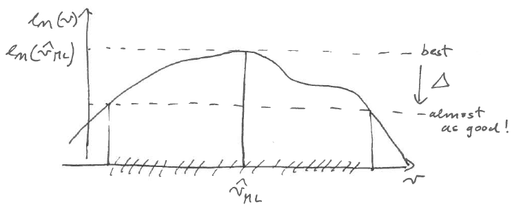
Idea: find all $\boldsymbol \theta_0$ that have a log-likelihood that is almost as good as $l_n(\hat{\boldsymbol \theta}_{ML} | D)$. \[\text{CI}= \{\boldsymbol \theta_0: l_n(\hat{\boldsymbol \theta}_{ML}| D) - l_n(\boldsymbol \theta_0 | D) \leq \Delta\}\] Here $\Delta$ is our tolerated deviation from the maximum log-likelihood. We will see below how to determine a suitable $\Delta$.

The above leads naturally to the Wilks log likelihood ratio statistic $W(\boldsymbol \theta_0)$ defined as: \[ \begin{split} W(\boldsymbol \theta_0) & = 2 \log \left(\frac{L(\hat{\boldsymbol \theta}_{ML}| D)}{L(\boldsymbol \theta_0| D)}\right) \\ & =2(l_n(\hat{\boldsymbol \theta}_{ML}| D)-l_n(\boldsymbol \theta_0 |D))\\ \end{split} \] With its help we can write the likelihood CI follows: \[\text{CI}= \{\boldsymbol \theta_0: W(\boldsymbol \theta_0) \leq 2 \Delta\}\]

The Wilks statistic is named after Samuel S. Wilks (1906–1964).

Advantages of using a likelihood-based CI:

not restricted to be symmetric
enables to construct multivariate CIs for parameter vector easily even in non-normal cases
contains normal CI as special case

Question: how to choose $\Delta$, i.e how to calibrate the likelihood interval?
Essentially, by comparing with a normal CI!

Example 5.1 Wilks statistic for the proportion:

The log-likelihood for the parameter $\theta$ is (cf. Example 3.1) \[ l_n(\theta| D) = n ( \bar{x} \log \theta + (1-\bar{x}) \log(1-\theta) ) \] Hence the Wilks statistic is \[ \begin{split} W(\theta_0) & = 2 ( l_n( \hat{\theta}_{ML} | D) -l_n( \theta_0 | D ) )\\ & = 2 n \left( \bar{x} \log \left( \frac{ \bar{x} }{\theta_0} \right) + (1-\bar{x}) \log \left( \frac{1-\bar{x} }{1-\theta_0} \right) \right) \\ \end{split} \]

Comparing with Example 2.8 we see that in this case the Wilks statistic is essentially (apart from a scale factor $2n$) the KL divergence between two Bernoulli distributions: \[ W(\theta_0) =2 n D_{\text{KL}}( \text{Ber}( \hat{\theta}_{ML} ), \text{Ber}(\theta_0) ) \]

Example 5.2 Wilks statistic for the mean parameter of a normal model:

The Wilks statistic is \[ W(\mu_0)^2 = \frac{(\bar{x}-\mu_0)^2}{\sigma^2 / n} \]

See Worksheet L3 for a derivation of the Wilks statistic directly from the log-likelihood function.

Note this is the same as the squared Wald statistic discussed in Example 4.6.

Comparing with Example 2.10 we see that in this case the Wilks statistic is essentially (apart from a scale factor $2n$) the KL divergence between two normal distributions with different means and variance equal to $\sigma^2$: \[ W(p_0) =2 n D_{\text{KL}}( N( \hat{\mu}_{ML}, \sigma^2 ), N(\mu_0, \sigma^2) ) \]

5.1.2 Quadratic approximation of Wilks statistic and squared Wald statistic

Recall the quadratic approximation of the log-likelihood function $l_n(\boldsymbol \theta_0| D)$ (= second order Taylor series around the MLE $\hat{\boldsymbol \theta}_{ML}$):

\[l_n(\boldsymbol \theta_0| D)\approx l_n(\hat{\boldsymbol \theta}_{ML}| D)-\frac{1}{2}(\boldsymbol \theta_0-\hat{\boldsymbol \theta}_{ML})^T \boldsymbol J_n(\hat{\boldsymbol \theta}_{ML}) (\boldsymbol \theta_0-\hat{\boldsymbol \theta}_{ML})\]

With this we can then approximate the Wilks statistic: \[ \begin{split} W(\boldsymbol \theta_0) & = 2(l_n(\hat{\boldsymbol \theta}_{ML}| D)-l_n(\boldsymbol \theta_0| D))\\ & \approx (\boldsymbol \theta_0-\hat{\boldsymbol \theta}_{ML})^T \boldsymbol J_n(\hat{\boldsymbol \theta}_{ML})(\boldsymbol \theta_0-\hat{\boldsymbol \theta}_{ML})\\ & =t(\boldsymbol \theta_0)^2 \\ \end{split} \]

Thus the quadratic approximation of the Wilks statistic yields the squared Wald statistic!

Conversely, the Wilks statistic can be understood a generalisation of the squared Wald statistic.

Example 5.3 Quadratic approximation of the Wilks statistic for a proportion (continued from Example 5.1):

A Taylor series of second order (for $p_0$ around $\bar{x}$) yields \[ \log \left( \frac{ \bar{x} }{p_0} \right) \approx -\frac{p_0-\bar{x}}{\bar{x}} + \frac{ ( p_0-\bar{x} )^2 }{2 \bar{x}^2 } \] and \[ \log \left( \frac{ 1- \bar{x} }{1- p_0} \right) \approx \frac{p_0-\bar{x}}{1-\bar{x}} + \frac{ ( p_0-\bar{x} )^2 }{2 (1-\bar{x})^2 } \] With this we can approximate the Wilks statistic of the proportion as \[ \begin{split} W(p_0) & \approx 2 n \left( - (p_0-\bar{x}) +\frac{ ( p_0-\bar{x} )^2 }{2 \bar{x} } + (p_0-\bar{x}) + \frac{ ( p_0-\bar{x} )^2 }{2 (1-\bar{x}) } \right) \\ & = n \left( \frac{ ( p_0-\bar{x} )^2 }{ \bar{x} } + \frac{ ( p_0-\bar{x} )^2 }{ (1-\bar{x}) } \right) \\ & = n \left( \frac{ ( p_0-\bar{x} )^2 }{ \bar{x} (1-\bar{x}) } \right) \\ &= t(p_0)^2 \,. \end{split} \] This verifies that the quadratic approximation of the Wilks statistic leads back to the squared Wald statistic of Example 4.5.

Example 5.4 Quadratic approximation of the Wilks statistic for the mean parameter of a normal model (continued from Example 5.2):

The normal log-likelihood is already quadratic in the mean parameter (cf. Example 3.2). Correspondingly, the Wilks statistic is quadratic in the mean parameter as well. Hence in this particular case the quadratic “approximation” is in fact exact and the Wilks statistic and the squared Wald statistic are identical!

Correspondingly, confidence intervals and tests based on the Wilks statistic are identical to those obtained using the Wald statistic.

5.1.3 Distribution of the Wilks statistic

The connection with the squared Wald statistic implies that both have asympotically the same distribution.

Hence, under $\boldsymbol \theta_0$ the Wilks statistic is distributed asymptotically as \[W(\boldsymbol \theta_0) \overset{a}{\sim} \chi^2_d\] where $d$ is the number of parameters in $\boldsymbol \theta$, i.e. the dimension of the model.

For scalar $\theta$ (i.e. single parameter and $d=1$) this becomes \[ W(\theta_0) \overset{a}{\sim} \chi^2_1 \]

This fact is known as Wilks’ theorem.

5.1.4 Cutoff values for the likelihood CI

coverage $\kappa$	$\Delta = \frac{c_{\text{chisq}}}{2}$ ($m=1$)
0.9	1.35
0.95	1.92
0.99	3.32

The asymptotic distribution for $W$ is useful to choose a suitable $\Delta$ for the likelihood CI — note that $2 \Delta = c_{\text{chisq}}$ where $c_{\text{chisq}}$ is the critical value for a specified coverage $\kappa$. This yields the above table for scalar parameter

Example 5.5 Likelihood confidence interval for a proportion:

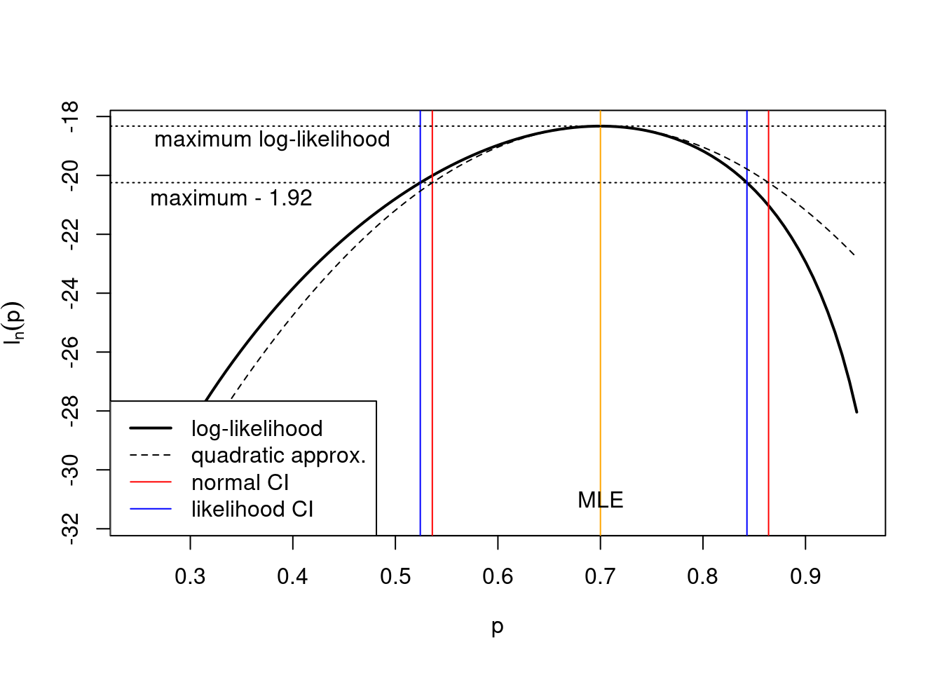
We continue from Example 5.1, and as in Example 4.7 we asssume we have data with $n = 30$ and $\bar{x} = 0.7$.

This yields (via numerical root finding) as the 95% likelihood confidence interval the interval $[0.524, 0.843]$. It is similar but not identical to the corresponding asymptotic normal interval $[0.536, 0.864]$ obtained in Example 4.7.

The following figure illustrate the relationship between the normal CI, the likelihood CI and also shows the role of the quadratic approximation (see also Example 4.2). Note that:

the normal CI is symmetric around the MLE whereas the likelihood CI is not symmetric
the normal CI is identical to the likelihood CI when using the quadratic approximation!

5.1.5 Likelihood ratio test (LRT) using Wilks statistic

As in the normal case (with Wald statistic and normal CIs) one can also construct a test using the Wilks statistic:

\[\begin{align*} \begin{array}{ll} H_0: \boldsymbol \theta= \boldsymbol \theta_0\\ H_1: \boldsymbol \theta\neq \boldsymbol \theta_0\\ \end{array} \begin{array}{ll} \text{ True model is } \boldsymbol \theta_0\\ \text{ True model is } \textbf{not } \boldsymbol \theta_0\\ \end{array} \begin{array}{ll} \text{ Null hypothesis}\\ \text{ Alternative hypothesis}\\ \end{array} \end{align*}\]

As test statistic we use the Wilks log likelihood ratio $W(\boldsymbol \theta_0)$. Extreme values of this test statistic imply evidence against $H_0$.

Note that the null model is “simple” (= a single parameter value) whereas the alternative model is “composite” (= a set of parameter values).

Remarks:

The composite alternative $H_1$ is represented by a single point (the MLE).
Reject $H_0$ for large values of $W(\boldsymbol \theta_0)$
under $H_0$ and for large $n$ the statistic $W(\boldsymbol \theta_0)$ is chi-squared distributed, i.e. $W(\boldsymbol \theta_0) \overset{a}{\sim} \chi^2_d$. This allows to compute critical values (i.e tresholds to declared rejection under a given significance level) and also $p$-values corresponding to the observed test statistics.
Models outside the CI are rejected
Models inside the CI cannot be rejected, i.e. they can’t be statistically distinguished from the best alternative model.

A statistic equivalent to $W(\boldsymbol \theta_0)$ is the likelihood ratio \[ \Lambda(\boldsymbol \theta_0) = \frac{L(\boldsymbol \theta_0| D)}{L(\hat{\boldsymbol \theta}_{ML}| D)} \] The two statistics can be transformed into each other by $W(\boldsymbol \theta_0) = -2\log \Lambda(\boldsymbol \theta_0)$ and $\Lambda(\boldsymbol \theta_0) = e^{ - W(\boldsymbol \theta_0) / 2 }$. We reject $H_0$ for small values of $\Lambda$.

It can be shown that the likelihood ratio test to compare two simple models is optimal in the sense that for any given specified type I error (=probability of wrongly rejecting $H_0$, i.e. the sigificance level) it will maximise the power (=1- type II error, probability of correctly accepting $H_1$). This is known as the Neyman-Pearson theorem.

Example 5.6 Likelihood test for a proportion:

We continue from Example 5.5 with 95% likelihood confidence interval $[0.524, 0.843]$.

The value $p_0=0.5$ is outside the CI and hence can be rejected whereas $p_0=0.8$ is insided the CI and hence cannot be rejected on 5% significance level.

The Wilks statistic for $p_0=0.5$ and $p_0=0.8$ takes on the following values:

$W(0.5) = 4.94 > 3.84$ hence $p_0=0.5$ can be rejected.
$W(0.8) = 1.69 < 3.84$ hence $p_0=0.8$ cannot be rejected.

Note that the Wilks statistic at the boundaries of the likelihood confidence interval is equal to the critical value (3.84 corresponding to 5% significance level for a chi-squared distribution with 1 degree of freedom).

Compare also with the normal test for a proportion in Example 4.9.

5.1.6 Origin of likelihood ratio statistic

The likelihood ratio statistic is asymptotically linked to differences in the KL divergences of the two compared models with the underlying true model.

Assume that $F$ is the true (and unknown) data generating model and that $G_{\boldsymbol \theta}$ is a family of models and we would like to compare two candidate models $G_A$ and $G_B$ corresponding to parameters $\boldsymbol \theta_A$ and $\boldsymbol \theta_B$ on the basis of observed data $D = \{x_1, \ldots, x_n\}$. The KL divergences $D_{\text{KL}}(F, G_A)$ and $D_{\text{KL}}(F, G_B)$ indicate how close each of the models $G_A$ and $G_B$ fit the true $F$. The difference of the two divergences is a way to measure the relative fit of the two models, and can be computed as \[ D_{\text{KL}}(F, G_B)-D_{\text{KL}}(F, G_A) = \text{E}_{F} \log \frac{g(x|\boldsymbol \theta_A )}{g(x| \boldsymbol \theta_B)} \] Replacing $F$ by the empirical distribution $\hat{F}_n$ leads to the large sample approximation \[ 2 n (D_{\text{KL}}(F, G_B)-D_{\text{KL}}(F, G_A)) \approx 2 (l_n(\boldsymbol \theta_A| D) - l_n(\boldsymbol \theta_B| D)) \] Hence, the difference in the log-likelihoods provides an estimate of the difference in the KL divergence of the two models involved.

The Wilks log likelihood ratio statistic \[ W(\boldsymbol \theta_0) = 2 ( l_n( \hat{\boldsymbol \theta}_{ML}| D ) - l_n(\boldsymbol \theta_0| D) ) \] thus compares the best-fit distribution with $\hat{\boldsymbol \theta}_{ML}$ as the parameter to the distribution with parameter $\boldsymbol \theta_0$.

For some specific models the Wilks statistic can also be written in the form of the KL divergence: \[ W(\boldsymbol \theta_0) = 2n D_{\text{KL}}( F_{\hat{\boldsymbol \theta}_{ML}}, F_{\boldsymbol \theta_0}) \] This is the case for the examples 5.1 and 5.2 and also more generally for exponential family models, but it is not true in general.

5.2 Generalised likelihood ratio test (GLRT)

Also known as maximum likelihood ratio test (MLRT). The Generalised Likelihood Ratio Test (GLRT) works just like the standard likelihood ratio test with the difference that now the null model $H_0$ is also a composite model.
\[\begin{align*} \begin{array}{ll} H_0: \boldsymbol \theta\in \omega_0 \subset \Omega \\ H_1: \boldsymbol \theta\in \omega_1 = \Omega \setminus \omega_0\\ \end{array} \begin{array}{ll} \text{ True model lies in restricted model space }\\ \text{ True model is not the restricted model space } \\ \end{array} \end{align*}\]

Both $H_0$ and $H_1$ are now composite hypotheses. $\Omega$ represents the unrestricted model space with dimension (=number of free parameters) $d = |\Omega|$. The constrained space $\omega_0$ has degree of freedom $d_0 = |\omega_0|$ with $d_0 < d$. Note that in the standard LRT the set $\omega_0$ is a simple point with $d_0=0$ as the null model is a simple distribution. Thus, LRT is contained in GLRT as special case!

The corresponding generalised (log) likelihood ratio statistic is given by

\[ W = 2\log\left(\frac{L(\hat{\theta}_{ML} |D )}{L(\hat{\theta}_{ML}^0 | D )}\right) \text{ and } \Lambda = \frac{\underset{\theta \in \omega_0}{\max}\, L(\theta| D)}{\underset{\theta \in \Omega}{\max}\, L(\theta | D)} \]

where $L(\hat{\theta}_{ML}| D)$ is the maximised likelihood assuming the full model (with parameter space $\Omega$) and $L(\hat{\theta}_{ML}^0| D)$ is the maximised likelihood for the restricted model (with parameter space $\omega_0$). Hence, to compute the GRLT test statistic we need to perform two optimisations, one for the full and another for the restricted model.

Remarks:

MLE in the restricted model space $\omega_0$ is taken as a representative of $H_0$.
The likelihood is maximised in both numerator and denominator.
The restricted model is a special case of the full model (i.e. the two models are nested).
The asymptotic distribution of $W$ is chi-squared with degree of freedom depending on both $d$ and $d_0$:

\[W \overset{a}{\sim} \text{$\chi^2_{d-d_0}$}\]

This result is due to Wilks (1938) ⁷. Note that it assumes that the true model is contained among the investigated models.
If $H_0$ is a simple hypothesis (i.e. $d_0=0$) then the standard LRT (and corresponding CI) is recovered as special case of the GLRT.

Example 5.7 GLRT example:

Case-control study: (e.g. “healthy” vs. “disease”)
we observe normal data $D = \{x_1, \ldots, x_n\}$ from two groups with sample size $n_1$ and $n_2$ (and $n=n_1+n_2$), with two different means $\mu_1$ and $\mu_2$ and common variance $\sigma^2$:

\[x_1,\dots,x_{n_1} \sim N(\mu_1, \sigma^2)\] and \[x_{n_1+1},\dots,x_{n} \sim N(\mu_2, \sigma^2)\]

Question: are the two means $\mu_1$ and $\mu_2$ the same in the two groups?

\[\begin{align*} \begin{array}{ll} H_0: \mu_1=\mu_2 \text{ (with variance unknown, i.e. treated as nuisance parameter)} \\ H_1: \mu_1\neq\mu_2\\ \end{array} \end{align*}\]

Restricted and full models:

$\omega_0$: restricted model with two parameters $\mu_0$ and $\sigma^2_0$ (so that $x_{1},\dots,x_{n} \sim N(\mu_0, \sigma_0^2)$ ).

$\Omega$: full model with three parameters $\mu_1, \mu_2, \sigma^2$.

Corresponding log-likelihood functions:

Restricted model $\omega_0$: \[ \log L(\mu_0, \sigma_0^2 | D) = -\frac{n}{2} \log(\sigma_0^2) - \frac{1}{2\sigma_0^2} \sum_{i=1}^n (x_i-\mu_0)^2 \]

Full model $\Omega$: \[ \begin{split} \log L(\mu_1, \mu_2, \sigma^2 | D) & = \left(-\frac{n_1}{2} \log(\sigma^2) - \frac{1}{2\sigma^2} \sum_{i=1}^{n_1} (x_i-\mu_1)^2 \right) + \\ & \phantom{==} \left(-\frac{n_2}{2} \log(\sigma^2) - \frac{1}{2\sigma^2} \sum_{i=n_1+1}^{n} (x_i-\mu_2)^2 \right) \\ &= -\frac{n}{2} \log(\sigma^2) - \frac{1}{2\sigma^2} \left( \sum_{i=1}^{n_1} (x_i-\mu_1)^2 + \sum_{i=n_1+1}^n (x_i-\mu_2)^2 \right) \\ \end{split} \]

Corresponding MLEs:

\[\begin{align*} \begin{array}{ll} \omega_0:\\ \\ \Omega:\\ \\ \end{array} \begin{array}{ll} \hat{\mu}_0 = \frac{1}{n}\sum^n_{i=1}x_i\\ \\ \hat{\mu}_1 = \frac{1}{n_1}\sum^{n_1}_{i=1}x_i\\ \hat{\mu}_2 = \frac{1}{n_2}\sum^{n}_{i=n_1+1}x_i\\ \end{array} \begin{array}{ll} \widehat{\sigma^2_0} = \frac{1}{n}\sum^n_{i=1}(x_i-\hat{\mu}_0)^2\\ \\ \widehat{\sigma^2} = \frac{1}{n}\left\{\sum^{n_1}_{i=1}(x_i-\hat{\mu}_1)^2+\sum^n_{i=n_1+1}(x_i-\hat{\mu}_2)^2\right\}\\ \\ \end{array} \end{align*}\]

Note that the estimated means are related by \[ \hat{\mu}_0 = \frac{n_1}{n} \hat{\mu}_1 + \frac{n_2}{n} \hat{\mu}_2 \] so the overall mean is the weighted average of the two individual group means.

Moreover, the two estimated variances are related by \[ \begin{split} \widehat{\sigma^2_0} & = \widehat{\sigma^2} + \frac{n_1 n_2}{n^2} (\hat{\mu}_1 - \hat{\mu}_2)^2\\ & = \widehat{\sigma^2} \left( 1+ \frac{1}{n} \frac{(\hat{\mu}_1 - \hat{\mu}_2)^2}{ \frac{n}{n_1 n_2} \widehat{\sigma^2}}\right) \\ & = \widehat{\sigma^2} \left( 1 + \frac{t^2_{ML}}{n}\right) \end{split} \] with \[ t_{ML} = \frac{\hat{\mu}_1-\hat{\mu}_2}{\sqrt{\left(\frac{1}{n_1}+\frac{1}{n_2}\right) \widehat{\sigma^2}}} \] (the $t$-statistic based on the ML variance estimate $\widehat{\sigma^2}$, see Appendix).

The above is an example of a variance decomposition, with

$\widehat{\sigma^2_0}$ being the estimated total variance,
$\widehat{\sigma^2}$ the estimated within-group variance and
$\widehat{\sigma^2}\frac{t^2_{ML}}{n}= \frac{n_1 n_2}{n^2} (\hat{\mu}_1 - \hat{\mu}_2)^2$ the estimated between-group variance.

and

$\frac{\widehat{\sigma^2}}{ \widehat{\sigma^2_0} } = 1 + \frac{t^2_{ML}}{n}$

Corresponding maximised log-likelihood:

Restricted model:

\[\log L(\hat{\mu}_0,\widehat{\sigma^2_0}| D) = -\frac{n}{2} \log(\widehat{\sigma^2_0}) -\frac{n}{2} \]

Full model:

\[ \log L(\hat{\mu}_1,\hat{\mu}_2,\widehat{\sigma^2}| D) = -\frac{n}{2} \log(\widehat{\sigma^2}) -\frac{n}{2} \]

Likelihood ratio statistic:

\[ \begin{split} W & = 2\log\left(\frac{L(\hat{\mu}_1,\hat{\mu}_2,\widehat{\sigma^2} | D)}{L(\hat{\mu}_0,\widehat{\sigma^2_0} | D)}\right)\\ & = 2 \log L\left(\hat{\mu}_1,\hat{\mu}_2,\widehat{\sigma^2}| D\right) - 2 \log L\left(\hat{\mu}_0,\widehat{\sigma^2_0}| D\right) \\ & = n\log\left(\frac{\widehat{\sigma^2_0}}{\widehat{\sigma^2}} \right) \\ & = n\log\left(1+\frac{t^2_{ML}}{n}\right) \\ \end{split} \] The last step uses the decomposition for the total variance $\widehat{\sigma^2_0}$.

We can express this also in terms of the conventional two sample $t$-statistic \[ t = \frac{\hat{\mu}_1-\hat{\mu}_2}{\sqrt{\left(\frac{1}{n_1}+\frac{1}{n_2}\right)\widehat{\sigma^2}_{\text{UB}} }} \] that uses an unbiased estimate of the variance rather than the MLE, with $\widehat{\sigma^2}_{\text{UB}}=\frac{n}{n-2} \widehat{\sigma^2}$ and thus $t^2/(n-2) = t^2_{ML} / n$. This yields \[ W=n\log\left(1+\frac{t^2}{n-2}\right) \]

Thus, the log-likelihood ratio statistic $W$ is a monotonic function (a one-to-one transformation!) of the (squared) two sample $t$-statistic!

Asymptotic distribution:

The degree of freedom of the full model is $d=3$ and that of the constrained model $d_0=2$ so the generalised log likelihood ratio statistic $W$ is distributed asymptotically as $\text{$\chi^2_{1}$}$. Hence, we reject the null model on 5% significance level for all $W > 3.84$.

Other application of GLRTs

As shown above, the two sample $t$ statistic can be derived as a likelihood ratio statistic.

More generally, it turns out many other commonly used familiar statistical tests and test statistics can be interpreted as GLRTs. This shows the wide applicability of this procedure.

4 Quadratic approximation and normal asymptotics

6 Optimality properties and conclusion