16 Estimating regression coefficients

In this chapter we discuss various ways to estimate the regression coefficients. First, we discuss estimation by Ordinary Least Squares (OLS) by minimising the residual sum of squares. This yields the famous Gauss estimator. Second, we derive estimates of the regression coefficients using the methods of maximum likelihood assuming normal errors. This also leads to the Gauss estimator. Third, we show that the coefficients in linear regression can written and interpreted in terms of two covariance matrices and that the Gauss estimator of the regression coefficients is a plug-in estimator using the MLEs of these covariance matrices. Furthermore, we show that the (population version) of the Gauss estimator can also be derived by finding the best linear predictor and by conditioning. Finally, we discuss special cases of regression coefficients and their relationship to marginal correlation.

16.1 Ordinary Least Squares (OLS) estimator of regression coefficients

Now we show the classic way (Gauss 1809; Legendre 1805) to estimate regression coefficients by the method of ordinary least squares (OLS).

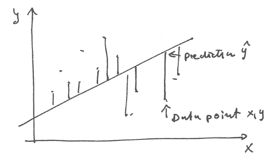
Idea: choose regression coefficients such as to minimise the squared error between observations and the prediction.

In data matrix notation (note we assume \(\beta_0=0\) and thus centered data \(\boldsymbol X\) and \(\boldsymbol y\)):

\[\text{RSS}(\boldsymbol \beta)=(\boldsymbol y-\boldsymbol X\boldsymbol \beta)^T(\boldsymbol y-\boldsymbol X\boldsymbol \beta)\]

RSS is an abbreviation for “Residual Sum of Squares” which is is a function of \(\boldsymbol \beta\). Minimising RSS yields the OLS estimate:

\[\widehat{\boldsymbol \beta}_{\text{OLS}}=\underset{\boldsymbol \beta}{\arg \min}\, \text{RSS}(\boldsymbol \beta)\]

\[\text{RSS}(\boldsymbol \beta) = \boldsymbol y^T \boldsymbol y- 2 \boldsymbol \beta^T \boldsymbol X^T \boldsymbol y+ \boldsymbol \beta^T \boldsymbol X^T \boldsymbol X\boldsymbol \beta\]

Gradient: \[\nabla \text{RSS}(\boldsymbol \beta) = -2\boldsymbol X^T \boldsymbol y+ 2\boldsymbol X^T \boldsymbol X\boldsymbol \beta\]

\[\nabla \text{RSS}(\widehat{\boldsymbol \beta}) = 0 \longrightarrow \boldsymbol X^T \boldsymbol y= \boldsymbol X^T\boldsymbol X\widehat{\boldsymbol \beta}\]

\[\Longrightarrow \widehat{\boldsymbol \beta}_{\text{OLS}} = \left(\boldsymbol X^T\boldsymbol X\right)^{-1} \boldsymbol X^T \boldsymbol y\]

Note the similarities in the procedure to maximum likelihood (ML) estimation (with minimisation instead of maximisation)! In fact, as we see next this is not by chance as OLS is indeed a special case of ML! This also implies that OLS is generally a good method — but only if sample size \(n\) is large!

The above Gauss’ estimator is fundamental in statistics so it is worthwile to memorise it!

16.2 Maximum likelihood estimation of regression coefficients

16.2.1 Normal log-likelihood function for regression coefficients and noise variance

We now show how to estimate regression coefficients using the method of maximum likelihood. This is a second method to derive \(\hat{\boldsymbol \beta}\).

We recall the basic regression equation \[ y = \beta_0 + \boldsymbol \beta^T \boldsymbol x+ \varepsilon \] with independent noise \(\varepsilon\) and observed data \(y_1, \ldots, y_n\) and \(\boldsymbol x_1, \ldots, \boldsymbol x_n\).

Assuming \(\text{E}(\varepsilon)=0\) the intercept is identified as \[ \beta_0 = \mu_{y}- \boldsymbol \beta^T \boldsymbol \mu_{\boldsymbol x} \] Combining the two above equations we see that noise variable equals \[ \varepsilon = (y- \mu_{y}) - \boldsymbol \beta^T (\boldsymbol x-\boldsymbol \mu_{\boldsymbol x}) \]

Assuming joint (multivariate) normality for the observed data, the response \(y\) and predictors \(\boldsymbol x\), we get as the MLEs for the respective means and (co)variances:

• \(\hat{\mu}_y=\hat{\text{E}}(y)= \frac{1}{n}\sum^n_{i=1} y_i\)
• \(\hat{\sigma}^2_y=\widehat{\text{Var}}(y)= \frac{1}{n}\sum^n_{i=1} (y_i - \hat{\mu}_y)^2\)
• \(\hat{\boldsymbol \mu}_{\boldsymbol x}=\hat{\text{E}}(\boldsymbol x)= \frac{1}{n}\sum^n_{i=1} \boldsymbol x_i\)
• \(\hat{\boldsymbol \Sigma}_{\boldsymbol x\boldsymbol x}=\widehat{\text{Var}}(\boldsymbol x)= \frac{1}{n}\sum^n_{i=1} (\boldsymbol x_i-\hat{\boldsymbol \mu}_{\boldsymbol x}) (\boldsymbol x_i-\hat{\boldsymbol \mu}_{\boldsymbol x})^T\)
• \(\hat{\boldsymbol \Sigma}_{\boldsymbol xy}=\widehat{\text{Cov}}(\boldsymbol x, y)= \frac{1}{n}\sum^n_{i=1} (\boldsymbol x_i-\hat{\boldsymbol \mu}_{\boldsymbol x}) (y_i - \hat{\mu}_y)\)

Note that these are are sufficient statistics and hence summarize perfectly the observed data for \(\boldsymbol x\) and \(y\) under the normal assumption

Consequently, the residuals (indirect observations of the noise variable) for a given choice of regression coefficients \(\boldsymbol \beta\) and the observed data for \(\boldsymbol x\) and \(y\) are \[ \varepsilon_i = (y_i- \hat{\mu}_{y}) - \boldsymbol \beta^T (\boldsymbol x_i -\hat{\boldsymbol \mu}_{\boldsymbol x}) \]

Assuming that the noise \(\varepsilon \sim N(0, \sigma^2_{\varepsilon})\) is normally distributed with mean 0 and variance \(\text{Var}(\varepsilon) = \sigma^2_{\varepsilon}\). we can write down the normal log-likelihood function for \(\sigma^2_{\varepsilon}\) and \(\boldsymbol \beta\): \[ \begin{split} \log L(\boldsymbol \beta,\sigma^2_{\varepsilon} ) &= -\frac{n}{2} \log \sigma^2_{\varepsilon} - \frac{1}{2\sigma^2_{\varepsilon}} \sum^n_{i=1} \left((y_i- \hat{\mu}_{y}) - \boldsymbol \beta^T (\boldsymbol x_i -\hat{\boldsymbol \mu}_{\boldsymbol x})\right)^2\\ \end{split} \] Maximising this function leads to the MLEs of \(\sigma^2_{\varepsilon}\) and \(\boldsymbol \beta\)!

Note that the residual sum of squares appears in the log-likelihood function (with a minus sign), which implies that ML assuming normal distribution will recover the OLS estimator for the regression coefficients! So OLS is a special case of ML !

16.2.2 Detailed derivation of the MLEs

The gradient with regard to \(\boldsymbol \beta\) is \[ \begin{split} \nabla_{\boldsymbol \beta} \log L(\boldsymbol \beta,\sigma^2_{\varepsilon} ) &= \frac{1}{\sigma^2_{\varepsilon}} \sum^n_{i=1} \left((\boldsymbol x_i -\hat{\boldsymbol \mu}_{\boldsymbol x} ) (y_i - \hat{\mu}_{y}) - (\boldsymbol x_i -\hat{\boldsymbol \mu}_{\boldsymbol x} )(\boldsymbol x_i -\hat{\boldsymbol \mu}_{\boldsymbol x})^T \boldsymbol \beta\right) \\ &= \frac{n}{\sigma^2_{\varepsilon}} \left( \hat{\boldsymbol \Sigma}_{\boldsymbol xy} - \hat{\boldsymbol \Sigma}_{\boldsymbol x\boldsymbol x}\boldsymbol \beta\right)\\ \end{split} \] Setting this equal to zero yields the Gauss estimator \[ \hat{\boldsymbol \beta} = \hat{\boldsymbol \Sigma}_{\boldsymbol x\boldsymbol x}^{-1} \hat{\boldsymbol \Sigma}_{\boldsymbol xy} \] By plugin we the get the MLE of \(\beta_0\) as \[ \hat{\beta}_0 = \hat{\mu}_{y}- \hat{\boldsymbol \beta}^T \hat{\boldsymbol \mu}_{\boldsymbol x} \] Taking the derivative of \(\log L(\hat{\boldsymbol \beta},\sigma^2_{\varepsilon} )\) with regard to \(\sigma^2_{\varepsilon}\) yields \[ \frac{\partial}{\partial \sigma^2_{\varepsilon}} \log L(\hat{\boldsymbol \beta},\sigma^2_{\varepsilon} ) = -\frac{n}{2\sigma^2_{\varepsilon}} +\frac{1}{2\sigma^4_{\varepsilon}} \sum^n_{i=1} (y_i-\hat{y}_i)^2 \] with \(\hat{y}_i = \hat{\beta}_0 + \hat{\boldsymbol \beta}^T \boldsymbol x_i\) and the residuals \(y_i-\hat{y}_i\) resulting from the fitted linear model. This leads to the MLE of the noise variance \[ \widehat{\sigma^2_{\varepsilon}} = \frac{1}{n}\sum^n_{i=1}(y_i-\hat{y}_i)^2 \]

Note that the MLE \(\widehat{\sigma^2_{\varepsilon}}\) is a biased estimate of \(\sigma^2_{\varepsilon}\). The unbiased estimate is \(\frac{1}{n-d-1}\sum^n_{i=1}(y_i-\hat{y}_i)^2\), where \(d\) is the dimension of \(\boldsymbol \beta\) (i.e. the number of predictors).

16.2.3 Asymptotics

The advantage of using maximum likelihood is that we also get the (asympotic) variance associated with each estimator and typically can also assume asymptotic normality.

Specifically, for \(\hat{\boldsymbol \beta}\) we get via the observed Fisher information at the MLE an asymptotic estimator of its variance \[\widehat{\text{Var}}(\widehat{\boldsymbol \beta})=\frac{1}{n} \widehat{\sigma^2_{\varepsilon}} \hat{\boldsymbol \Sigma}_{\boldsymbol x\boldsymbol x}^{-1}\] Similarly, for \(\hat{\beta}_0\) we have \[ \widehat{\text{Var}}(\widehat{\beta}_0)=\frac{1}{n} \widehat{\sigma^2_{\varepsilon}} (1 + \hat{\boldsymbol \mu}^T \hat{\boldsymbol \Sigma}_{\boldsymbol x\boldsymbol x}^{-1} \hat{\boldsymbol \mu}) \]

For finite sample size \(n\) with known \(\text{Var}(\varepsilon)\) one can show that the variances are \[\text{Var}(\widehat{\boldsymbol \beta})=\frac{1}{n} \sigma^2_{\varepsilon}\hat{\boldsymbol \Sigma}_{\boldsymbol x\boldsymbol x}^{-1}\] and \[ \text{Var}(\widehat{\beta}_0)=\frac{1}{n} \sigma^2_{\varepsilon} (1 + \hat{\boldsymbol \mu}^T_{\boldsymbol x} \hat{\boldsymbol \Sigma}_{\boldsymbol x\boldsymbol x}^{-1} \hat{\boldsymbol \mu}_{\boldsymbol x}) \] and that the regression coefficients and the intercept are normally distributed according to \[ \widehat{\boldsymbol \beta} \sim N_d(\boldsymbol \beta, \text{Var}(\widehat{\boldsymbol \beta})) \] and \[ \widehat{\beta}_0 \sim N(\beta_0, \text{Var}(\widehat{\beta}_0)) \]

We may use this to test whether whether \(\beta_j = 0\) and \(\beta_0 = 0\).

16.3 Covariance plug-in estimator of regression coefficients

16.3.1 Regression coeffients as product of variances

We now try to understand regression coefficients in terms of covariances (thus obtaining a third way to compute and estimate them).

We recall that the Gauss regression coefficients are given by

\[\widehat{\boldsymbol \beta} = \left(\boldsymbol X^T\boldsymbol X\right)^{-1}\boldsymbol X^T \boldsymbol y\] where \(\boldsymbol X\) is the \(n \times d\) data matrix (in statistics convention)

\[\boldsymbol X= \begin{pmatrix} x_{11} & \dots & x_{1d} \\ \vdots & \ddots & \vdots \\ x_{n1} & \dots & x_{nd} \end{pmatrix}\] Note that we assume that the data matrix \(\boldsymbol X\) is centered (i.e. column sums \(\boldsymbol X^T \boldsymbol 1_n = \boldsymbol 0\) are zero).

Likewise \(\boldsymbol y= (y_1, \ldots, y_n)^T\) is the response data vector (also centered with \(\boldsymbol y^T \boldsymbol 1_n = 0\)).

Noting that \[\hat{\boldsymbol \Sigma}_{\boldsymbol x\boldsymbol x}=\frac{1}{n}(\boldsymbol X^T\boldsymbol X)\] is the MLE of covariance matrix among \(\boldsymbol x\) and \[\hat{\boldsymbol \Sigma}_{\boldsymbol xy}=\frac{1}{n}(\boldsymbol X^T \boldsymbol y)\] is the MLE of the covariance between \(\boldsymbol x\) and \(y\) we see that the OLS estimate of the regression coefficients can be expressed as \[\widehat{\boldsymbol \beta} = \left(\hat{\boldsymbol \Sigma}_{\boldsymbol x\boldsymbol x}\right)^{-1}\hat{\boldsymbol \Sigma}_{\boldsymbol xy}\] We can write down a population version (with no hats!): \[\boldsymbol \beta= \boldsymbol \Sigma_{\boldsymbol x\boldsymbol x}^{-1} \boldsymbol \Sigma_{\boldsymbol xy}\]

Thus, OLS regression coefficients can be interpreted as plugin estimator using MLEs of covariances! In fact, we may also use the unbiased estimates since the scale factor (\(1/n\) or \(1/(n-1)\)) cancels out so it does not matter which one you use!

16.3.2 Importance of positive definiteness of estimated covariance matrix

Note that \(\hat{\boldsymbol \Sigma}_{\boldsymbol x\boldsymbol x}\) is inverted in \(\widehat{\boldsymbol \beta} = \left(\hat{\boldsymbol \Sigma}_{\boldsymbol x\boldsymbol x}\right)^{-1}\hat{\boldsymbol \Sigma}_{\boldsymbol xy}\).

• Hence, the estimate \(\hat{\boldsymbol \Sigma}_{\boldsymbol x\boldsymbol x}\) needs to be positive definite!
• But \(\hat{\boldsymbol \Sigma}_{\boldsymbol x\boldsymbol x}^{\text{MLE}}\) is only positive definite if \(n>d\)!

Therefore we can use the ML estimate (empirical estimator) only for large \(n\) > \(d\), otherwise we need to employ a different (regularised) estimation approach (e.g. Bayes or a penalised ML)!

Remark: writing \(\hat{\boldsymbol \beta}\) explicitly based on covariance estimates has the advantage that we can construct plug-in estimators of regression coefficients based on regularised covariance estimators that improve over ML for small sample size. This leads to the so-called SCOUT method (=covariance-regularized regression by Witten and Tibshirani, 2008).

16.4 Standardised regression coefficients and their relationship to correlation

We recall the relationship between regression coefficients \(\boldsymbol \beta\) and the marginal covariance \(\boldsymbol \Sigma_{\boldsymbol xy}\) and the covariances among the predictors \(\boldsymbol \Sigma_{\boldsymbol x\boldsymbol x}\):

\[\boldsymbol \beta= \boldsymbol \Sigma_{\boldsymbol x\boldsymbol x}^{-1} \boldsymbol \Sigma_{\boldsymbol xy}\]

We can rewrite the regression coefficients in terms of marginal correlations \(\boldsymbol P_{\boldsymbol xy}\) and correlations \(\boldsymbol P_{\boldsymbol x\boldsymbol x}\) among the predictors using the variance-correlation decompositions \(\boldsymbol \Sigma_{\boldsymbol x\boldsymbol x}= \boldsymbol V_{\boldsymbol x}^{1/2} \boldsymbol P_{\boldsymbol x\boldsymbol x} \boldsymbol V_{\boldsymbol x}^{1/2}\) and \(\boldsymbol \Sigma_{\boldsymbol xy}= \boldsymbol V_{\boldsymbol x}^{1/2} \boldsymbol P_{\boldsymbol xy} \sigma_y\): \[ \begin{split} \boldsymbol \beta&= \underbrace{\boldsymbol V_{\boldsymbol x}^{-1/2}}_{\text{(inverse) scale of } x_i} \,\, \boldsymbol P_{\boldsymbol x\boldsymbol x}^{-1} \boldsymbol P_{\boldsymbol xy} \,\, \underbrace{\sigma_y}_{\text{ scale of }y} \\ &= \boldsymbol V_{\boldsymbol x}^{-1/2} \,\, \boldsymbol \beta_{\text{std}} \,\, \sigma_y \\ \end{split} \] Thus the regression coefficients \(\boldsymbol \beta\) contain the scale of the variables, and take into account the correlations among the predictors (\(\boldsymbol P_{\boldsymbol x\boldsymbol x}\)) in addition to the marginal correlations between the response \(y\) and the predictors \(x_i\) (\(\boldsymbol P_{\boldsymbol xy}\)).

This decomposition allows to understand a number special cases for which the regression coefficients simplify further:

1. If the response and the predictors are standardised to have variance one, i.e. \(\text{Var}(y)=1\) and \(\text{Var}(x_i)=1\), then \(\boldsymbol \beta\) becomes equal to the standardised regression coefficients \[\boldsymbol \beta_{\text{std}} = \boldsymbol P_{\boldsymbol x\boldsymbol x}^{-1} \boldsymbol P_{\boldsymbol xy}\] Note that standardised regression coefficients do not make use of variances and and thus are scale-independent.

2. If there is no correlation among the predictors , i.e. \(\boldsymbol P_{\boldsymbol x\boldsymbol x} = \boldsymbol I\) the the regression coefficients reduce to \[\boldsymbol \beta= \boldsymbol V_{\boldsymbol x}^{-1} \boldsymbol \Sigma_{\boldsymbol xy}\] where \(\boldsymbol V_{\boldsymbol x}\) is a diagonal matrix containing the variances of the predictors. This is also called marginal regression. Note that the inversion of \(\boldsymbol V_{\boldsymbol x}\) is trival since you only need to invert each diagonal element individually.

3. If both a) and b) apply simultaneously (i.e. there is no correlation among predictors and response and predictors and predictors are standardised) then the regression coefficients simplify even further to \[ \boldsymbol \beta= \boldsymbol P_{\boldsymbol xy} \] Thus, in this very special case the regression coefficients are identical to the correlations between the response and the predictors!

16.5 Further ways to obtain regression coefficients

16.5.1 Best linear predictor

The best linear predictor is a fourth way to arrive at the linear model. This is closely related to OLS and minimising squared residual error.

Without assuming normality the above multiple regression model can be shown to be optimal linear predictor under the minimum mean squared prediction error:

Assumptions:

• \(y\) and \(\boldsymbol x\) are random variables
• we construct a new variable (the linear predictor) \(y^{\star\star} = b_0 + \boldsymbol b^T \boldsymbol x\) to optimally approximate \(y\)

Aim:

• choose \(b_0\) and \(\boldsymbol b\) such to minimize the mean squared prediction error \(\text{E}( (y - y^{\star\star})^2 )\)

16.5.1.1 Result:

The mean squared prediction error \(MSPE\) in dependence of \((b_0, \boldsymbol b)\) is \[ \begin{split} \text{E}( (y - y^{\star\star} )^2) & = \text{Var}(y - y^{\star\star}) + \text{E}(y - y^{\star\star})^2 \\ & = \text{Var}(y - b_0 -\boldsymbol b^T \boldsymbol x) + ( \text{E}(y) -b_0 - \boldsymbol b^T \text{E}(\boldsymbol x) )^2 \\ & = \sigma^2_y + \text{Var}(\boldsymbol b^T \boldsymbol x) + 2 \, \text{Cov}(y, -\boldsymbol b^T \boldsymbol x) + ( \mu_y -b_0 - \boldsymbol b^T \boldsymbol \mu_{\boldsymbol x} )^2 \\ & = \sigma^2_y + \boldsymbol b^T \boldsymbol \Sigma_{\boldsymbol x\boldsymbol x} \boldsymbol b- 2 \, \boldsymbol b^T \boldsymbol \Sigma_{\boldsymbol xy} + ( \mu_y -b_0 - \boldsymbol b^T \boldsymbol \mu_{\boldsymbol x} )^2 \\ & = MSPE(b_0, \boldsymbol b) \\ \end{split} \]

We look for \[ (\beta_0, \boldsymbol \beta) = \underset{b_0,\boldsymbol b}{\arg\min} \,\, MSPE(b_0, \boldsymbol b) \]

In order to find the minimum we compute the gradient with regard to \((b_0, \boldsymbol b)\) \[ \nabla MSPE = \begin{pmatrix} -2( \mu_y -b_0 - \boldsymbol b^T \boldsymbol \mu_{\boldsymbol x} ) \\ 2 \, \boldsymbol \Sigma_{\boldsymbol x\boldsymbol x} \boldsymbol b- 2 \, \boldsymbol \Sigma_{\boldsymbol xy} -2 \boldsymbol \mu_{\boldsymbol x} (\mu_y -b_0 - \boldsymbol b^T \boldsymbol \mu_{\boldsymbol x}) \\ \end{pmatrix} \] and setting this equal to zero yields \[ \begin{pmatrix} \beta_0\\ \boldsymbol \beta\\ \end{pmatrix} = \begin{pmatrix} \mu_y- \boldsymbol \beta^T \boldsymbol \mu_{\boldsymbol x} \\ \boldsymbol \Sigma_{\boldsymbol x\boldsymbol x}^{-1} \boldsymbol \Sigma_{\boldsymbol xy}\\ \end{pmatrix} \] Thus, the optimal values for \(b_0\) and \(\boldsymbol b\) in the best linear predictor correspond to the previously derived coefficients \(\beta_0\) and \(\boldsymbol \beta\)!

16.5.1.2 Irreducible Error

The minimum achieved MSPE (=irreducible error) is \[ MSPE(\beta_0,\boldsymbol \beta) = \sigma^2_{y} - \boldsymbol \beta^T \boldsymbol \Sigma_{\boldsymbol x\boldsymbol x} \boldsymbol \beta= \sigma^2_{y} - \boldsymbol \Sigma_{y \boldsymbol x} \boldsymbol \Sigma_{\boldsymbol x\boldsymbol x}^{-1} \boldsymbol \Sigma_{\boldsymbol xy} \] With the abbreviation \(\Omega^2 = \boldsymbol P_{y \boldsymbol x} \boldsymbol P_{\boldsymbol x\boldsymbol x}^{-1} \boldsymbol P_{\boldsymbol xy} = \sigma_y^{-2} \boldsymbol \Sigma_{y \boldsymbol x} \boldsymbol \Sigma_{\boldsymbol x\boldsymbol x}^{-1} \boldsymbol \Sigma_{\boldsymbol xy}\) we can simplify this to \[ MSPE(\beta_0,\boldsymbol \beta) = \sigma^2_y (1-\Omega^2) = \text{Var}(\varepsilon) \]

Writing \(b_0=\beta_0 + \Delta_0\) and \(\boldsymbol b= \boldsymbol \beta+ \boldsymbol \Delta\) it is easy to see that the mean squared predictive error is a quadratic function around the minimum: \[ MSPE(\beta_0 + \Delta_0, \boldsymbol \beta+ \boldsymbol \Delta) = \text{Var}(\varepsilon) + \Delta_0^2 + \boldsymbol \Delta^T \boldsymbol \Sigma_{\boldsymbol x\boldsymbol x} \boldsymbol \Delta \]

Note that usually \(y^{\star} = \beta_0 + \boldsymbol \beta^T \boldsymbol x\) does not perfectly approximate \(y\) so there will be an irreducible error (= noise variance) \[\text{Var}(\varepsilon) =\sigma^2_y (1-\Omega^2) > 0\] which implies \(\Omega^2 < 1\).

The quantity \(\Omega^2\) has a further interpretation of the population version of as the squared multiple correlation coefficient between the response and the predictors and plays a vital role in decomposition of variance, as discussed later.

16.5.2 Regression by conditioning

Conditioning is a fifth way to arrive at the linear model. This is also the most general way and can be used to derive many other regression models (not just the simple linear model).

16.5.2.1 General idea:

• two random variables \(y\) (response, scalar) and \(\boldsymbol x\) (predictor variables, vector)
• we assume that \(y\) and \(\boldsymbol x\) have a joint distribution \(F_{y,\boldsymbol x}\)
• compute conditional random variable \(y | \boldsymbol x\) and the corresponding distribution \(F_{y | \boldsymbol x}\)

16.5.2.2 Multivariate normal assumption

Now we assume that \(y\) and \(\boldsymbol x\) are (jointly) multivariate normal. Then the conditional distribution \(F_{y | \boldsymbol x}\) is a univariate normal with the following moments (you can verify this by looking up the general conditional multivariate normal distribution):

a) Conditional expectation:

\[ \text{E}( y | \boldsymbol x) = y^{\star} = \beta_0 + \boldsymbol \beta^T \boldsymbol x\]

with coefficients \(\boldsymbol \beta= \boldsymbol \Sigma_{\boldsymbol x\boldsymbol x}^{-1}\boldsymbol \Sigma_{\boldsymbol xy}\) and intercept \(\beta_0 = \mu_{y} - \boldsymbol \beta^T \boldsymbol \mu_{\boldsymbol x}\) .

Note that as \(y^{\star}\) depends on \(\boldsymbol x\) it is a random variable itself with mean \[ \text{E}(y^{\star}) = \beta_0 + \boldsymbol \beta^T \boldsymbol \mu_{\boldsymbol x} = \mu_{y} \] and variance \[ \begin{split} \text{Var}(y^{\star}) & = \text{Var}(\text{E}( y | \boldsymbol x)) \\ & = \boldsymbol \beta^T \boldsymbol \Sigma_{\boldsymbol x\boldsymbol x} \boldsymbol \beta= \boldsymbol \Sigma_{y \boldsymbol x} \boldsymbol \Sigma_{\boldsymbol x\boldsymbol x}^{-1} \boldsymbol \Sigma_{\boldsymbol xy} \\ & = \sigma^2_y \boldsymbol P_{y \boldsymbol x} \boldsymbol P_{\boldsymbol x\boldsymbol x}^{-1} \boldsymbol P_{\boldsymbol xy} \\ & = \sigma_y^2 \Omega^2\\ \end{split} \]

b) Conditional variance:

\[ \begin{split} \text{Var}( y | \boldsymbol x) &=\sigma^2_y - \boldsymbol \beta^T \boldsymbol \Sigma_{\boldsymbol x\boldsymbol x} \boldsymbol \beta\\ & = \sigma^2_y - \boldsymbol \Sigma_{y \boldsymbol x} \boldsymbol \Sigma_{\boldsymbol x\boldsymbol x}^{-1} \boldsymbol \Sigma_{\boldsymbol xy} \\ & = \sigma^2_y (1-\Omega^2)\\ \end{split} \] Note this is a constant so \(\text{E}(\text{Var}( y | \boldsymbol x)) = \sigma^2_y (1-\Omega^2)\) as well.