A Refresher

Statistics is a mathematical science that requires practical use of tools from probability, vector and matrices, analysis etc.

Here we briefly list some essentials that are needed for “Statistical Methods”. Please familiarise yourself (again) with these topics.

A.1 Basic mathematical notation

Summation: \[ \sum_{i=1}^n x_i = x_1 + x_2 + \ldots + x_n \]

Multiplication: \[ \prod_{i=1}^n x_i = x_1 \times x_2 \times \ldots \times x_n \]

A.2 Vectors and matrices

Vector and matrix notation.

Vector algebra.

Eigenvectors and eigenvalues for a real symmetric matrix.

Eigenvalue (spectral) decomposition of a real symmetric matrix.

Positive and negative definiteness of a real symmetric matrix (containing only positive or only negative eigenvalues).

Singularity of a real symmetric matrix (containing one or more eigenvalues identical to zero).

Singular value decomposition of a real matrix.

Inverse of a matrix.

Trace and determinant of a square matrix.

Connection with eigenvalues (trace = sum of eigenvalues, determinant = product of eigenvalues).

A.3 Functions

A.3.1 Gradient

The gradient of a scalar-valued function \(h(\boldsymbol x)\) with vector argument \(\boldsymbol x= (x_1, \ldots, x_d)^T\) is the vector containing the first order partial derivatives of \(h(\boldsymbol x)\) with regard to each \(x_1, \ldots, x_d\): \[ \begin{split} \nabla h(\boldsymbol x) &= \begin{pmatrix} \frac{\partial h(\boldsymbol x)}{\partial x_1} \\ \vdots\\ \frac{\partial h(\boldsymbol x)}{\partial x_d} \end{pmatrix}\\ &= \frac{\partial h(\boldsymbol x)}{\partial \boldsymbol x} \\ & = \text{grad } h(\boldsymbol x) \\ \end{split} \] The symbol \(\nabla\) is called the nabla operator (also known as del operator).

Note that we write the gradient as a column vector. This is called the denominator layout convention, see https://en.wikipedia.org/wiki/Matrix_calculus for details. In contrast, many textbooks (and also earlier versions of these lecture notes) assume that gradients are row vectors, following the so-called numerator layout convention.

Example A.1 Examples for the gradient:

• \(h(\boldsymbol x)=\boldsymbol a^T \boldsymbol x+ b\). Then \(\nabla h(\boldsymbol x) = \frac{\partial h(\boldsymbol x)}{\partial \boldsymbol x} = \boldsymbol a\).
• \(h(\boldsymbol x)=\boldsymbol x^T \boldsymbol x\). Then \(\nabla h(\boldsymbol x) = \frac{\partial h(\boldsymbol x)}{\partial \boldsymbol x} = 2 \boldsymbol x\).
• \(h(\boldsymbol x)=\boldsymbol x^T \boldsymbol A\boldsymbol x\). Then \(\nabla h(\boldsymbol x) = \frac{\partial h(\boldsymbol x)}{\partial \boldsymbol x} = (\boldsymbol A+ \boldsymbol A^T) \boldsymbol x\).

A.3.2 Hessian matrix

The matrix of all second order partial derivates of scalar-valued function with vector-valued argument is called the Hessian matrix: \[ \begin{split} \nabla \nabla^T h(\boldsymbol x) &= \begin{pmatrix} \frac{\partial^2 h(\boldsymbol x)}{\partial x_1^2} & \frac{\partial^2 h(\boldsymbol x)}{\partial x_1 \partial x_2} & \cdots & \frac{\partial^2 h(\boldsymbol x)}{\partial x_1 \partial x_d} \\ \frac{\partial^2 h(\boldsymbol x)}{\partial x_2 \partial x_1} & \frac{\partial^2 h(\boldsymbol x)}{\partial x_2^2} & \cdots & \frac{\partial^2 h(\boldsymbol x)}{\partial x_2 \partial x_d} \\ \vdots & \vdots & \ddots & \vdots \\ \frac{\partial^2 h(\boldsymbol x)}{\partial x_d \partial x_1} & \frac{\partial^2 h(\boldsymbol x)}{\partial x_d \partial x_2} & \cdots & \frac{\partial^2 h(\boldsymbol x)}{\partial x_d^2} \end{pmatrix} \\ &= \left(\frac{\partial h(\boldsymbol x)}{\partial x_i \partial x_j}\right) \\ & = \frac{\partial^2 h(\boldsymbol x)}{\partial \boldsymbol x\partial \boldsymbol x^T} \\ \end{split} \] By construction the Hessian matrix is square and symmetric.

Example A.2 \(h(\boldsymbol x)=\boldsymbol x^T \boldsymbol A\boldsymbol x\). Then \(\nabla \nabla^T h(\boldsymbol x) = \frac{\partial^2 h(\boldsymbol x)}{\partial \boldsymbol x\partial \boldsymbol x^T} = (\boldsymbol A+ \boldsymbol A^T)\).

A.3.3 Convex and concave functions

A function \(h(x)\) is convex if the second derivative \(h''(x) \geq 0\) for all \(x\). More generally, a function \(h(\boldsymbol x)\), where \(\boldsymbol x\) is a vector, is convex if the Hessian matrix \(\nabla \nabla^T h(\boldsymbol x)\) is positive definite, i.e. if the eigenvalues of the Hessian matrix are all positive.

If \(h(\boldsymbol x)\) is convex, then \(-h(\boldsymbol x)\) is concave. A function is concave if the Hessian matrix is negative definite, i.e. if the eigenvalues of the Hessian matrix are all negative.

Example A.3 The logarithm \(\log(x)\) is an example of a concave function whereas \(x^2\) is a convex function.

To memorise, a valley is convex.

A.3.4 Linear and quadratic approximation

A linear and quadratic approximation of a function is given by a Taylor series of first and second order, respectively.

Applied to scalar-valued function of a scalar: \[ h(x) \approx h(x_0) + h'(x_0) (x-x_0) + \frac{1}{2} h''(x_0) (x-x_0)^2 \] Note that \(h'(x_0) = h'(x) \,|\, x_0\) is first derivative of \(h(x)\) evaluated at \(x_0\) and \(h''(x_0) = h''(x) \,|\, x_0\) is the second derivative of \(h(x)\) evaluated \(x_0\).

With \(x = x_0+ \varepsilon\) the approximation can also be written as \[ h(x_0+ \varepsilon) \approx h(x_0) + h'(x_0) \, \varepsilon + \frac{1}{2} h''(x_0)\, \varepsilon^2 \]

Applied to scalar-valued function of a vector: \[ h(\boldsymbol x) \approx h(\boldsymbol x_0) + \nabla h(\boldsymbol x_0)^T (\boldsymbol x-\boldsymbol x_0) + \frac{1}{2} (\boldsymbol x-\boldsymbol x_0)^T \, \nabla \nabla^T h(\boldsymbol x_0) \, (\boldsymbol x-\boldsymbol x_0) \] Note that \(\nabla h(\boldsymbol x_0)\) is the gradient of \(h(\boldsymbol x)\) evaluated at \(\boldsymbol x_0\) and \(\nabla \nabla^T h(\boldsymbol x_0)\) the Hessian matrix of \(h(\boldsymbol x)\) evaluated at \(\boldsymbol x_0\).

With \(\boldsymbol x= \boldsymbol x_0+ \boldsymbol \varepsilon\) this approximation can also be written as \[ h(\boldsymbol x_0+ \boldsymbol \varepsilon) \approx h(\boldsymbol x_0) + \nabla h(\boldsymbol x_0)^T\boldsymbol \varepsilon+ \frac{1}{2} \boldsymbol \varepsilon^T \, \nabla \nabla^T h(\boldsymbol x_0) \,\boldsymbol \varepsilon \]

Example A.4 Commonly occurring Taylor series approximations of second order are for example \[ \log(x_0+\varepsilon) \approx \log(x_0) + \frac{\varepsilon}{x_0} - \frac{\varepsilon^2}{2 x_0^2} \] and \[ \frac{x_0}{x_0+\varepsilon} \approx 1 - \frac{\varepsilon}{x_0} + \frac{\varepsilon^2}{ x_0^2} \]

A.3.5 Conditions for local optimum of a function

To check if \(x_0\) or \(\boldsymbol x_0\) is a local maximum or minimum we can use the following conditions:

For a function of a single variable:

1. First derivative is zero at optimum \(h'(x_0) = 0\).
2. If the second derivative \(h''(x_0) < 0\) at the optimum is negative the function is locally concave and the optimum is a maximum.
3. If the second derivative \(h''(x_0) > 0\) is positive at the optimum the function is locally convex and the optimum is a minimum.

For a function of several variables:

1. Gradient vanishes at maximum, \(\nabla h(\boldsymbol x_0)=0\).
2. If the Hessian \(\nabla \nabla^T h(\boldsymbol x_0)\) is negative definite (= all eigenvalues of Hessian matrix are negative) then the function is locally concave and the optimum is a maximum.
3. If the Hessian is positive definite (= all eigenvalues of Hessian matrix are positive) then the function is locally convex and the optimum is a minimum.

Around the local optimum \(\boldsymbol x_0\) we can approximate the function quadratically using \[ h(\boldsymbol x_0+ \boldsymbol \varepsilon) \approx h(\boldsymbol x_0) + \frac{1}{2} \boldsymbol \varepsilon^T \nabla \nabla^T h(\boldsymbol x_0) \boldsymbol \varepsilon \] Note the linear term is missing due to the gradient being zero at \(\boldsymbol x_0\).

A.4 Combinatorics

A.4.1 Number of permutations

The number of possible orderings, or permutations, of \(n\) distinct items is the number of ways to put \(n\) items in \(n\) bins with exactly one item in each bin. It is given by the factorial \[ n! = \prod_{i=1}^n i = 1 \times 2 \times \ldots \times n \] where \(n\) is a positive integer. For \(n=0\) the factorial is defined as \[ 0! = 1 \] as there is exactly one permutation of zero objects.

The factorial can also be obtained using the gamma function \[ \Gamma(x) = \int_0^\infty t^{x-1} e^{-t} dt \] which can be viewed as continuous version of the factorial with \(\Gamma(x) = (x-1)!\) for any positive integer \(x\).

A.4.2 Multinomial and binomial coefficient

The number of possible permutation of \(n\) items of \(K\) distinct types, with \(n_1\) of type 1, \(n_2\) of type 2 and so on, equals the number of ways to put \(n\) items into \(K\) bins with \(n_1\) items in the first bin, \(n_2\) in the second and so on. It is given by the multinomial coefficient \[ \binom{n}{n_1, \ldots, n_K} = \frac {n!}{n_1! \times n_2! \times\ldots \times n_K! } \] with \(\sum_{k=1}^K n_k = n\) and \(K \leq n\). Note that it equals the number of permutation of all items divided by the number of permutations of the items in each bin (or of each type).

If all \(n_k=1\) and hence \(K=n\) the multinomial coefficient reduces to the factorial.

If there are only two bins / types (\(K=2\)) the multinomial coefficients becomes the binomial coefficient \[ \binom{n}{n_1} = \binom{n}{n_1, n-n_1} = \frac {n!}{n_1! (n - n_1)!} \] which counts the number of ways to choose \(n_1\) elements from a set of \(n\) elements.

A.4.3 De Moivre-Sterling approximation of the factorial

The factorial is frequently approximated by the following formula derived by Abraham de Moivre (1667–1754) and James Stirling (1692-1770) \[ n! \approx \sqrt{2 \pi} n^{n+\frac{1}{2}} e^{-n} \] or equivalently on logarithmic scale \[ \log n! \approx \left(n+\frac{1}{2}\right) \log n -n + \frac{1}{2}\log \left( 2 \pi\right) \] The approximation is good for small \(n\) (but fails for \(n=0\)) and becomes more and more accurate with increasing \(n\). For large \(n\) the approximation can be simplified to \[ \log n! \approx n \log n -n \]

A.5 Probability

A.5.1 Random variables

A random variable describes a random experiment. The set of possible outcomes is the sample space or state space and is denoted by \(\Omega = \{\omega_1, \omega_2, \ldots\}\). The outcomes \(\omega_i\) are the elementary events. The sample space \(\Omega\) can be finite or infinite. Depending on type of outcomes the random variable is discrete or continuous.

An event \(A \subseteq \Omega\) is subset of \(\Omega\) and thus itself a set of elementary events \(A = \{a_1, a_2, \ldots\}\). This includes as special cases the full set \(A = \Omega\), the empty set \(A = \emptyset\), and the elementary events \(A=\omega_i\). The complementary event \(A^C\) is the complement of the set \(A\) in the set \(\Omega\) so that \(A^C = \Omega \setminus A = \{\omega_i \in \Omega: \omega_i \notin A\}\).

The probability of an event is denoted by \(\text{Pr}(A)\). We assume that

• \(\text{Pr}(A) \geq 0\), probabilities are positive,
• \(\text{Pr}(\Omega) = 1\), the certain event has probability 1, and
• \(\text{Pr}(A) = \sum_{a_i \in A} \text{Pr}(a_i)\), the probability of an event equals the sum of its constituting elementary events \(a_i\).

This implies

• \(\text{Pr}(A) \leq 1\), i.e. probabilities all lie in the interval \([0,1]\)
• \(\text{Pr}(A^C) = 1 - \text{Pr}(A)\), and
• \(\text{Pr}(\emptyset) = 0\)

Assume now we have two events \(A\) and \(B\). The probability of the event “\(A\) and \(B\)” is then given by the probability of the set intersection \(\text{Pr}(A \cap B)\). Likewise the probability of the event “\(A\) or \(B\)” is given by the probability of the set union \(\text{Pr}(A \cup B)\).

From the above it is clear that probability theory is closely linked to set theory, and in particular to measure theory. This allows for an unified treatment of discrete and continuous random variables (an elegant framework but not needed for this module).

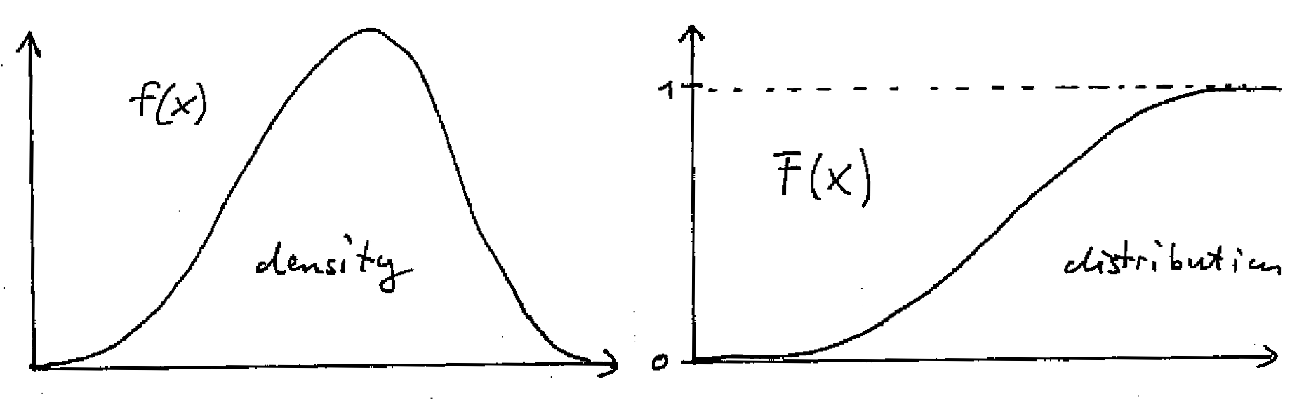
A.5.2 Probability mass and density function and distribution and quantile function

To describe a random variable \(x\) we need to assign probabilities to the corresponding elementary outcomes \(x \in \Omega\). For convenience we use the same name to denote the random variable and the elementary outcomes.

For a discrete random variable we employ a probability mass function (PMF). We denote the it by a lower case \(f\) but occasionally we also use \(p\) or \(q\). In the discrete case we can define the event \(A = \{x: x=a\} = \{a\}\) and obtain the probability directly from the PMF: \[\text{Pr}(A) = \text{Pr}(x=a) =f(a) \,.\] The PMF has the property that \(\sum_{x \in \Omega} f(x) = 1\) and that \(f(x) \in [0,1]\).

For continuous random variables we need to use a probability density function (PDF) instead. We define the event \(A = \{x: a < x \leq a + da\}\) as an infinitesimal interval and then assign the probability \[ \text{Pr}(A) = \text{Pr}( a < x \leq a + da) = f(a) da \,. \] The PDF has the property that \(\int_{x \in \Omega} f(x) dx = 1\) but in contrast to a PMF the density \(f(x)\geq 0\) may take on values larger than 1.

Assuming an ordering we can define the event \(A = \{x: x \leq a \}\) and compute its probability \[ F(a) = \text{Pr}(A) = \text{Pr}( x \leq a ) = \begin{cases} \sum_{x \in A} f(x) & \text{discrete case} \\ \int_{x \in A} f(x) dx & \text{continuous case} \\ \end{cases} \] This is known as the distribution function, or cumulative distribution function (CDF) and is denoted by upper case \(F\) if the corresponding PDF/PMF is \(f\) (or \(P\) and \(Q\) if the corresponding PDF/PMF are \(p\) and \(q\)). By construction the distribution function is monotonically increasing and its value ranges from 0 to 1. With its help we can compute the probability of general interval sets such as \[ \text{Pr}( a < x \leq b ) = F(b)-F(a) \,. \]

The inverse of the distribution function \(y=F(x)\) is the quantile function \(x=F^{-1}(y)\). The 50% quantile \(F^{-1}\left(\frac{1}{2}\right)\) is the median.

If the random variable \(x\) has distribution function \(F\) we write \(x \sim F\).

A.5.3 Expection and variance of a random variable

The expected value \(\text{E}(x)\) of a random variable is defined as the weighted average over all possible outcomes, with the weight given by the PMF / PDF \(f(x)\): \[ \text{E}(x) = \begin{cases} \sum_{x \in \Omega} f(x) x & \text{discrete case} \\ \int_{x \in \Omega} f(x) x dx & \text{continuous case} \\ \end{cases} \] To emphasise that the expecation is taken with regard to the distribution \(F\) we write \(\text{E}_F(x)\) with the distribution \(F\) as subscript. The expectation is not necessarily always defined for a continuous random variable as the integral may diverge.

The expected value of a function of a random variable \(h(x)\) is obtained similarly: \[ \text{E}(h(x)) = \begin{cases} \sum_{x \in \Omega} f(x) h(x) & \text{discrete case} \\ \int_{x \in \Omega} f(x) h(x) dx & \text{continuous case} \\ \end{cases} \] This is called the “law of the unconscious statistician”, or short LOTUS. Again, to highlight that the random variable \(x\) has distribution \(F\) we write \(\text{E}_F(h(x))\).

For an event \(A\) we can define a corresponding indicator function \[ 1_A(x) = \begin{cases} 1 & x \in A\\ 0 & x \notin A\\ \end{cases} \] Intriguingly, \[ \text{E}(1_A(x) ) = \text{Pr}(A) \] i.e. the expectation of the indicator variable for \(A\) is the probability of \(A\).

The moments of random variables are also defined by expectation:

• Zeroth moment: \(\text{E}(x^0) = 1\) by definition of PDF and PMF,
• First moment: \(\text{E}(x^1) = \text{E}(x) = \mu\) , the mean,
• Second moment: \(\text{E}(x^2)\)
• The variance is the second momented centered about the mean \(\mu\): \[\text{Var}(x) = \text{E}( (x - \mu)^2 ) = \sigma^2\]
• The variance can also be computed by \(\text{Var}(x) = \text{E}(x^2)-\text{E}(x)^2\).

A distribution does not necessarily need to have any finite first or higher moments. An example is the Cauchy distribution that does not have a mean or variance (or any other higher moment).

A.5.4 Transformation of random variables

Linear transformation of random variables: if \(a\) and \(b\) are constants and \(x\) is a random variable, then the random variable \(y= a + b x\) has mean \(\text{E}(y) = a + b \text{E}(x)\) and variance \(\text{Var}(y) = b^2 \text{Var}(x)\).

For a general invertible coordinate transformation \(y = h(x) = y(x)\) the backtransformation is \(x = h^{-1}(y) = x(y)\).

The transformation of the infinitesimal volume element is \(dy = |\frac{dy}{dx}| dx\).

The transformation of the density is \(f_y(y) =\left|\frac{dx}{dy}\right| f_x(x(y))\).

Note that \(\left|\frac{dx}{dy}\right| = \left|\frac{dy}{dx}\right|^{-1}\).

A.5.5 Law of large numbers:

Suppose we observe data \(D=\{x_1, \ldots, x_n\}\) with each \(x_i \sim F\).

• By the strong law of large numbers the empirical distribution \(\hat{F}_n\) based on data \(D=\{x_1, \ldots, x_n\}\) converges to the true underlying distribution \(F\) as \(n \rightarrow \infty\) almost surely: \[ \hat{F}_n\overset{a. s.}{\to} F \] The Glivenko–Cantelli theorem asserts that the convergence is uniform. Since the strong law implies the weak law we also have convergence in probability: \[ \hat{F}_n\overset{P}{\to} F \]

• Correspondingly, for \(n \rightarrow \infty\) the average \(\text{E}_{\hat{F}_n}(h(x)) = \frac{1}{n} \sum_{i=1}^n h(x_i)\) converges to the expectation \(\text{E}_{F}(h(x))\).

A.5.6 Jensen’s inequality

\[\text{E}(h(\boldsymbol x)) \geq h(\text{E}(\boldsymbol x))\] for a convex function \(h(\boldsymbol x)\).

Recall: a convex function (such as \(x^2\)) has the shape of a “valley”.

A.6 Distributions

A.6.1 Bernoulli distribution and binomial distribution

The Bernoulli distribution \(\text{Ber}(\theta)\) is simplest distribution possible. It is named after Jacob Bernoulli (1655-1705) who also invented the law of large numbers.

It describes a discrete binary random variable with two states \(x=0\) (“failure”) and \(x=1\) (“success”), where the parameter \(\theta \in [0,1]\) is the probability of “success”. Often the Bernoulli distribution is also referred to as “coin tossing” model with the two outcomes “heads” and “tails”.

Correspondingly, the probability mass function of \(\text{Ber}(\theta)\) is \[ p(x=0) = \text{Pr}(\text{"failure"}) = 1-\theta \] and \[ p(x=1) = \text{Pr}(\text{"success"}) = \theta \] A compact way to write the PMF of the Bernoulli distribution is \[ p(x | \theta ) = \theta^{x} (1-\theta)^{1-x} \]

If a random variable \(x\) follows the Bernoulli distribution we write \[ x \sim \text{Ber}(\theta) \,. \] The expected value is \(\text{E}(x) = \theta\) and the variance is \(\text{Var}(x) = \theta (1 - \theta)\).

Closely related to the Bernoulli distribution is the binomial distribution \(\text{Bin}(n, \theta)\) which results from repeating a Bernoulli experiment \(n\) times and counting the number of successes among the \(n\) trials (without keeping track of the ordering of the experiments). Thus, if \(x_1, \ldots, x_n\) are \(n\) independent \(\text{Ber}(\theta)\) random variables then \(y = \sum_{i=1}^n\) is distributed as \(\text{Bin}(n, \theta)\).

Its probability mass function is: \[ p(y | n, \theta) = \binom{n}{y} \theta^y (1 - \theta)^{n - y} \] for \(y \in \{ 0, 1, 2, \ldots, n\}\). The binomial coefficient \(\binom{n}{x}\) is needed to account for the multiplicity of ways (orderings of samples) in which we can observe \(y\) sucesses.

The expected value is \(\text{E}(y) = n \theta\) and the variance is \(\text{Var}(y) = n \theta (1 - \theta)\).

If a random variable \(y\) follows the binomial distribution we write \[ y \sim \text{Bin}(n, \theta)\, \] For \(n=1\) it reduces to the Bernoulli distribution \(\text{Ber}(\theta)\).

In R the PMF of the binomial distribution is called dbinom(). The binomial coefficient itself is computed by choose().

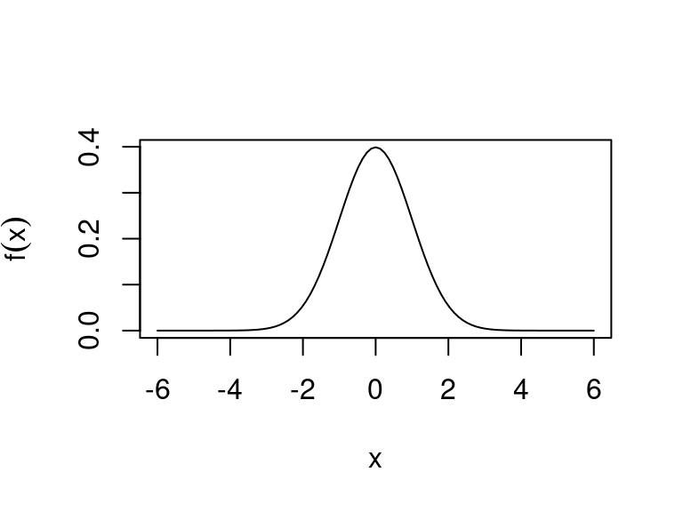
A.6.2 Normal distribution

The normal distribution is the most important continuous probability distribution. It is also called Gaussian distribution named after Carl Friedrich Gauss (1777–1855).

The univariate normal distribution \(N(\mu, \sigma^2)\) has two parameters \(\mu\) (location) and \(\sigma^2\) (scale):

\[ x \sim N(\mu,\sigma^2) \] with mean \[ \text{E}(x)=\mu \] and variance \[ \text{Var}(x) = \sigma^2 \]

Probability density function (PDF): \[ p(x| \mu, \sigma^2)=(2\pi\sigma^2)^{-\frac{1}{2}}\exp\left(-\frac{(x-\mu)^2}{2\sigma^2}\right) \]

In R the density function is called dnorm().

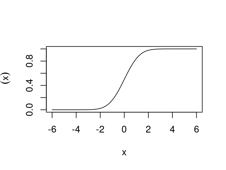
The standard normal distribution is \(N(0, 1)\) with mean 0 and variance 1.

Plot of the PDF of the standard normal:

The cumulative distribution function (CDF) of the standard normal \(N(0,1)\) is \[ \Phi (x ) = \int_{-\infty}^{x} f(x'| \mu=0, \sigma^2=1) dx' \] There is no analytic expression for \(\Phi(x)\). In R the function is called pnorm().

Plot of the CDF of the standard normal:

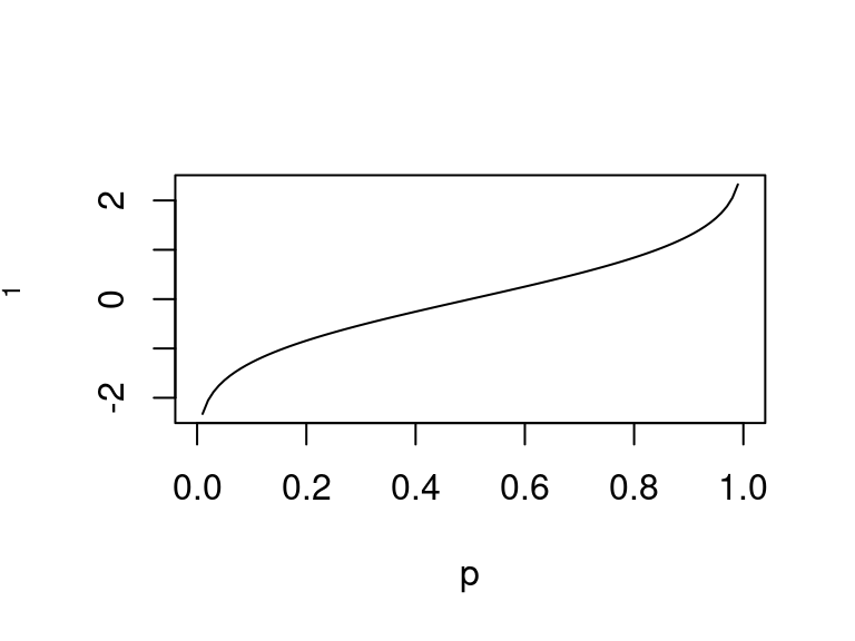
The inverse \(\Phi^{-1}(p)\) is called the quantile function of the standard normal. In R the function is called qnorm().

The sum of two normal random variables is also normal (with the appropriate mean and variance).

The central limit theorem (first postulated by Abraham de Moivre (1667–1754)) asserts that in many cases the distribution of the mean of identically distributed independent random variables converges to a normal distribution, even if the individual random variables are not normal.

A.6.3 Gamma distribution

A.6.3.1 Standard parameterisation

Another important continous distribution is the gamma distribution \(\text{Gam}(\alpha, \theta)\). It has two parameters \(\alpha>0\) (shape) and \(\theta>0\) (scale): \[ x \sim\text{Gam}(\alpha, \theta) \] with mean \[\text{E}(x)=\alpha \theta\] and variance \[\text{Var}(x) = \alpha \theta^2\]

The gamma distribution is also often used with a rate parameter \(\beta=1/\theta\) (so one needs to pay attention which parameterisation is used).

Probability density function (PDF): \[ p(x| \alpha, \theta)=\frac{1}{\Gamma(\alpha) \theta^{\alpha} } x^{\alpha-1} e^{-x/\theta} \] The density of the gamma distribution is available in the R function dgamma(). The cumulative density function is pgamma() and the quantile function is qgamma().

A.6.3.2 Wishart parameterisation and scaled chi-squared distribution

The gamma distribution is often used with a different set of parameters \(k=2 \alpha\) and \(s^2 =\theta/2\) (hence conversely \(\alpha = k/2\) and \(\theta=2 s^2\)). In this form it is known as one-dimensional Wishart distribution \[ W_1\left(s^2, k \right) \] named after John Wishart (1898–1954). In the Wishart parameterisation the mean is \[ \text{E}(x) = k s^2 \] and the variance \[ \text{Var}(x) = 2 k s^4 \]

Another name for the one-dimensional Wishart distribution with exactly the same parameterisation is scaled chi-squared distribution denoted as \[ s^2 \text{$\chi^2_{k}$} \]

Finally, note we often employ the Wishart distribution in mean parameterisation \(W_1\left(s^2= \mu / k, k \right)\) with \(\mu = k s^2\) and \(k\) (and thus \(\theta = 2 \mu /k\)). It has mean \[ \text{E}(x) = \mu \] and variance \[ \text{Var}(x) = \frac{2 \mu^2}{k} \]

A.6.3.3 Construction as sum of squared normals

A gamma distributed variable can be constructed as follows. Assume \(k\) independent normal random variables with mean 0 and variance \(s^2\): \[z_1,z_2,\dots,z_k\sim N(0,s^2)\] Then the sum of the squares \[ x = \sum_{i=1}^{k} z_i^2 \] follows \[ x \sim \sigma^2 \text{$\chi^2_{k}$} = W_1\left( s^2, k \right) \] or equivalently \[ x \sim \text{Gam}\left(\alpha=\frac{k}{2}, \theta = 2 s^2\right) \]

A.6.4 Special cases of the gamma distribution

A.6.4.1 Chi-squared distribution

The chi-squared distribution \(\text{$\chi^2_{k}$}\) is a special one-parameter restriction of the gamma resp. Wishart distribution obtained when setting \(s^2=1\) or, equivalently, \(\theta = 2\) or \(\mu = k\).

It has mean \(\text{E}(x)=k\) and variance \(\text{Var}(x)=2k\). The chi-squared distribution \(\text{$\chi^2_{k}$}\) equals \(\text{Gam}(\alpha=k/2, \theta=2) = W_1\left(1, k \right)\).

Here is a plot of the density of the chi-squared distribution for degrees of freedom \(k=1\) and \(k=3\):

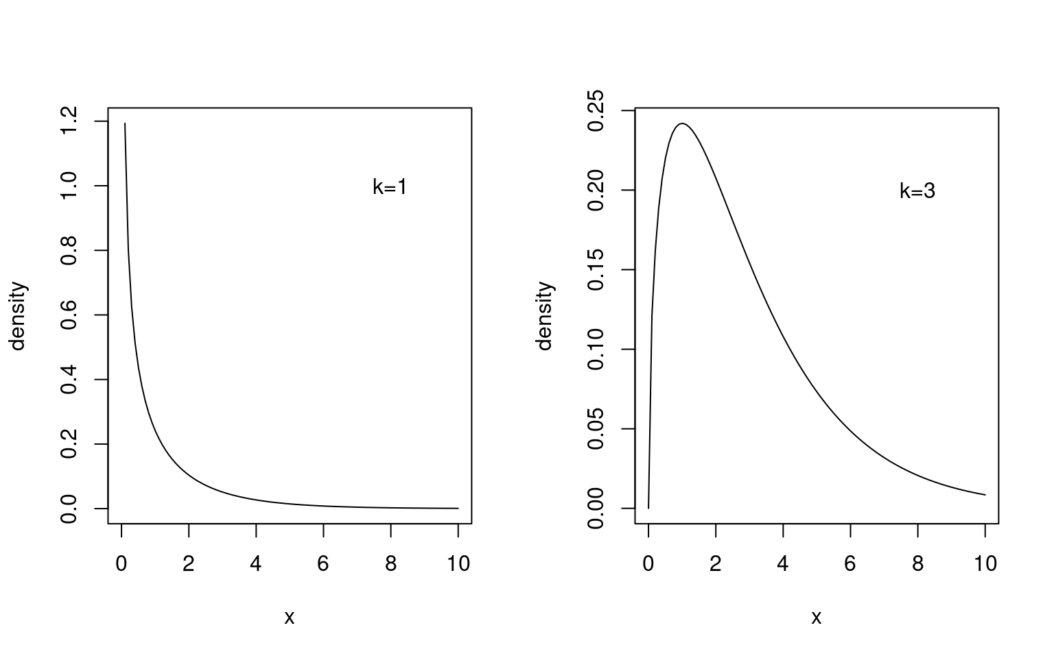
In R the density of the chi-squared distribution is given by dchisq(). The cumulative density function is pchisq() and the quantile function is qchisq().

A.6.4.2 Exponential distribution

The exponential distribution \(\text{Exp}(\theta)\) with scale parameter \(\theta\) is another special one-parameter restriction of the gamma distribution with shape parameter set to \(\alpha=1\) (or equivalently \(k=2\)).

It thus equals \(\text{Gam}(\alpha=1, \theta) = W_1(s^2=\theta/2, k=2)\). It has mean \(\theta\) and variance \(\theta^2\).

Just like the gamma distribution the exponential distribution is also often specified using a rate parameter \(\beta= 1/\theta\) instead of a scale parameter \(\theta\).

In R the command dexp() returns the density of the exponential distribution, pexp() is the corresponding cumulative density function and qexp() is the quantile function.

A.6.5 Location-scale \(t\)-distribution, Student’s \(t\)-distribution and Cauchy distribution

A.6.5.1 Location-scale \(t\)-distribution

The location-scale \(t\)-distribution \(\text{lst}(\mu, \tau^2, \nu)\) is a generalisation of the normal distribution. It has an additional parameter \(\nu > 0\) (degrees of freedom) that controls the probability mass in the tails. For small values of \(\nu\) the distribution is heavy-tailed — indeed so heavy that for \(\nu \leq 1\) even the mean is not defined and for \(\nu \leq 2\) the variance is undefined.

The probability density of \(\text{lst}(\mu, \tau^2, \nu)\) is \[ p(x | \mu, \tau^2, \nu) = \frac{\Gamma(\frac{\nu+1}{2})} {\sqrt{\pi \nu \tau^2} \,\Gamma(\frac{\nu}{2})} \left(1+\frac{(x-\mu)^2}{\nu \tau^2} \right)^{-(\nu+1)/2} \] The mean is (for \(\nu>1\)) \[ \text{E}(x) = \mu \] and the variance (for \(\nu>2\)) \[ \text{Var}(x) = \tau^2 \frac{\nu}{\nu-2} \]

For \(\nu \rightarrow \infty\) the location-scale \(t\)-distribution \(\text{lst}(\mu, \tau^2, \nu)\) becomes the normal distribution \(N(\mu, \tau^2)\).

For \(\nu=1\) the location-scale \(t\)-distribution becomes the Cauchy distribution \(\text{Cau}(\mu, \tau)\) with density \(p(x| \mu, \tau) = \frac{\tau}{\pi (\tau^2+(x-\mu)^2)}\).

In the R extraDistr package the command dlst() returns the density of the location-scale \(t\)-distribution, plst() is the corresponding cumulative density function and qlst() is the quantile function.

A.6.5.2 Student’s \(t\)-distribution

For \(\mu=0\) and \(\tau^2=1\) the location-scale \(t\)-distribution becomes the Student’s \(t\)-distribution \(t_\nu\) with mean 0 (for \(\nu>1\)) and variance \(\frac{\nu}{\nu-2}\) (for \(\nu>2\)).

If \(y \sim t_\nu\) then \(x = \mu + \tau y\) is distributed as \(x \sim \text{lst}(\mu, \tau^2, \nu)\).

For \(\nu \rightarrow \infty\) the \(t\)-distribution becomes equal to \(N(0,1)\).

For \(\nu=1\) the \(t\)-distribution becomes the standard Cauchy distribution \(\text{Cau}(0, 1)\) with density \(p(x) = \frac{1}{\pi (1+x^2)}\).

In R the command dt() returns the density of the \(t\)-distribution, pt() is the corresponding cumulative density function and qt() is the quantile function.

A.7 Statistics

A.7.1 Statistical learning

The aim in statistics — data science — machine learning is to use data (from experiments, observations, measurements) to learn about and understand the world.

Specifically, the aim is to identify the best model(s) for the data in order to

• to explain the current data, and
• to enable good prediction of future data

Note that it is easy to find models that explain the data but do not predict well!

Typically, one would like to avoid overfitting the data and prefers models that are appropriate for the data at hand (i.e. not too simple but also not too complex).

Specifically, data are denoted \(D =\{x_1, \ldots, x_n\}\) and models \(p(x| \theta)\) that are indexed the parameter \(\theta\).

Often (but not always) \(\theta\) can be interpreted and/or is associated with some property of the model.

If there is only a single parameter we write \(\theta\) (scalar parameter). For a parameter vector we write \(\boldsymbol \theta\) (in bold type).

A.7.2 Point and interval estimation

• There is a parameter \(\theta\) of interest in a model
• we are uncertain about this parameter (i.e. we don’t know the exact value)
• we would like to learn about this parameter by observing data \(x_1, \ldots, x_n\) from the model

Often the parameter(s) of interest are related to moments (such as mean and variance) or to quantiles of the distribution representing the model.

Estimation:

• An estimator for \(\theta\) is a function \(\hat{\theta}(x_1, \ldots, x_n)\) that maps the data (input) to a “guess” (output) about \(\theta\).
• A point estimator provides a single number for each parameter
• An interval estimator provides a set of possible values for each parameter.

Simple estimators of mean and variance:

Suppose we have data \(D = \{x_1, \ldots, x_n\}\) all sampled independently from a distribution \(F\).

• The average (also known as empirical mean) \(\hat{\mu} = \frac{1}{n} \sum_{i=1}^n x_i\) is an estimate of the mean of \(F\).
• The empirical variance \(\widehat{\sigma^2}_{\text{ML}} = \frac{1}{n} \sum_{i=1}^n (x_i -\hat{\mu})^2\) is an estimate of the variance of \(F\). Note the factor \(1/n\). It is the maximum likelihood estimate assuming a normal model.
• The unbiased sample variance \(\widehat{\sigma^2}_{\text{UB}} = \frac{1}{n-1} \sum_{i=1}^n (x_i -\hat{\mu})^2\) is another estimate of the variance of \(F\). Note the factor \(1/(n-1)\) therefore \(n\geq 2\) is required for this estimator.

A.7.3 Sampling properties of a point estimator \(\hat{\boldsymbol \theta}\)

A point estimator \(\hat\theta\) depends on the data, hence it has sampling variation (i.e. estimate will be different for a new set of observations)

Thus \(\hat\theta\) can be seen as a random variable, and its distribution is called sampling distribution (across different experiments).

Properties of this distribution can be used to evaluate how far the estimator deviates (on average across different experiments) from the true value:

\[\begin{align*} \begin{array}{rr} \text{Bias:}\\ \text{Variance:}\\ \text{Mean squared error:}\\ \\ \end{array} \begin{array}{rr} \text{Bias}(\hat{\theta})\\ \text{Var}(\hat{\theta})\\ \text{MSE}(\hat{\theta})\\ \\ \end{array} \begin{array}{ll} =\text{E}(\hat{\theta})-\theta\\ =\text{E}\left((\hat{\theta}-\text{E}(\hat{\theta}))^2\right)\\ =\text{E}((\hat{\theta}-\theta)^2)\\ =\text{Var}(\hat{\theta})+\text{Bias}(\hat{\theta})^2\\ \end{array} \end{align*}\]

The last identity about MSE follows from \(\text{E}(x^2)=\text{Var}(x)+\text{E}(x)^2\).

At first sight it seems desirable to focus on unbiased (for finite \(n\)) estimators. However, requiring strict unbiasedness is not always a good idea!

In many situations it is better to allow for some small bias and in order to achieve a smaller variance and an overall total smaller MSE. This is called bias-variance tradeoff — as more bias is traded for smaller variance (or, conversely, less bias is traded for higher variance)

A.7.4 Consistency

Typically, \(\text{Bias}\), \(\text{Var}\) and \(\text{MSE}\) all decrease with increasing sample size so that with more data \(n \to \infty\) the errors become smaller and smaller.

The typical rate of decrease of variance of a good estimator is \(\frac{1}{n}\). Thus, when sample size is doubled the variance is divided by 2 (and the standard deviation is divided by \(\sqrt{2}\)).

Consistency: \(\hat{\theta}\) is called consistent if \[ \text{MSE}(\hat{\theta}) \longrightarrow 0 \text{ with $n\rightarrow \infty$ } \] The three estimators discussed above (empirical mean, empirical variance, unbiased variance) are all consistent as their MSE goes to zero with large sample size \(n\).

Consistency is a minimum essential requirement for any reasonable estimator! Of all consistent estimators we typically prefer the estimator that is most efficient (i.e. with fasted decrease in MSE) and that therefore has smallest variance and/or MSE for given finite \(n\).

Consistency implies we recover the true model in the limit of infinite data if the model class contains the true data generating model.

If the model class does not contain the true model then strict consistency cannot be achived but we still wish to get as close as possible to the true model when choosing model parameters.

A.7.5 Sampling distribution of mean and variance estimators for normal data

Suppose we have data \(x_1, \ldots, x_n\) all sampled from a normal distribution \(N(\mu, \sigma^2)\).

• The empirical estimator of the mean parameter \(\mu\) is given by \(\hat{\mu} = \frac{1}{n} \sum_{i=1}^n x_i\). Under the normal assumption the distribution of \(\hat{\mu}\) is \[ \hat{\mu} \sim N\left(\mu, \frac{\sigma^2}{n}\right) \] Thus \(\text{E}(\hat{\mu}) = \mu\) and \(\text{Var}(\hat{\mu}) = \frac{\sigma^2}{n}\). The estimate \(\hat{\mu}\) is unbiased since \(\text{E}(\hat{\mu})-\mu = 0\) The mean squared error of \(\hat{\mu}\) is \(\text{MSE}(\hat{\mu}) = \frac{\sigma^2}{n}\).

• The empirical variance \(\widehat{\sigma^2}_{\text{ML}} = \frac{1}{n} \sum_{i=1}^n (x_i -\hat{\mu})^2\) for normal data follows a one-dimensional Wishart distribution \[ \widehat{\sigma^2}_{\text{ML}} \sim W_1\left(s^2 = \frac{\sigma^2}{n}, k=n-1\right) \] Thus, \(\text{E}( \widehat{\sigma^2}_{\text{ML}} ) = \frac{n-1}{n}\sigma^2\) and \(\text{Var}( \widehat{\sigma^2}_{\text{ML}} ) = \frac{2(n-1)}{n^2}\sigma^4\). The estimate \(\widehat{\sigma^2}_{\text{ML}}\) is biased since \(\text{E}( \widehat{\sigma^2}_{\text{ML}} )-\sigma^2 = -\frac{1}{n}\sigma^2\). The mean squared error is \(\text{MSE}( \widehat{\sigma^2}_{\text{ML}} ) = \frac{2(n-1)}{n^2}\sigma^4 +\frac{1}{n^2}\sigma^4 =\frac{2 n-1}{n^2}\sigma^4\).

• The unbiased variance estimate \(\widehat{\sigma^2}_{\text{UB}} = \frac{1}{n-1} \sum_{i=1}^n (x_i -\hat{\mu})^2\) for normal data follows a one-dimensional Wishart distribution \[ \widehat{\sigma^2}_{\text{UB}} \sim W_1\left(s^2 = \frac{\sigma^2}{n-1}, k = n-1 \right) \] Thus, \(\text{E}( \widehat{\sigma^2}_{\text{UB}} ) = \sigma^2\) and \(\text{Var}( \widehat{\sigma^2}_{\text{UB}} ) = \frac{2}{n-1}\sigma^4\). The estimate \(\widehat{\sigma^2}_{\text{ML}}\) is unbiased since \(\text{E}( \widehat{\sigma^2}_{\text{UB}} )-\sigma^2 =0\). The mean squared error is \(\text{MSE}( \widehat{\sigma^2}_{\text{UB}} ) =\frac{2}{n-1}\sigma^4\).

  Interestingly, for any \(n>1\) we find that \(\text{Var}( \widehat{\sigma^2}_{\text{UB}} ) > \text{Var}( \widehat{\sigma^2}_{\text{ML}} )\) and \(\text{MSE}( \widehat{\sigma^2}_{\text{UB}} ) > \text{MSE}( \widehat{\sigma^2}_{\text{ML}} )\) so that the biased empirical estimator has both lower variance and lower mean squared error than the unbiased estimator.

A.7.6 One sample \(t\)-statistic

Supppose we observe \(n\) independent data points \(x_1, \ldots, x_n \sim N(\mu, \sigma^2)\). Then the average \(\bar{x} = \sum_{i=1}^n x_i\) is distributed as \(\bar{x} \sim N(\mu, \sigma^2/n)\) and correspondingly \[ z = \frac{\bar{x}-\mu}{\sqrt{\sigma^2/n}} \sim N(0, 1) \]

Note that \(z\) uses the known variance \(\sigma^2\). If instead the variance is estimated by \(s^2_{\text{UB}} = \frac{1}{n-1} \sum_{i=1}^n (x_i -\bar{x})^2\) then the one sample \(t\)-statistic \[ t = \frac{\bar{x}-\mu}{\sqrt{s^2_{\text{UB}}/n}} \sim t_{n-1} \] is obtained. It is distributed according to a Student’s \(t\)-distribution with \(n-1\) degrees of freedom, with mean 0 for \(n>2\) and variance \((n-1)/(n-3)\) for \(n>3\).

If instead of the unbiased estimate the empirical (ML) estimate of the variance \(s^2_{\text{ML}} = \frac{1}{n} \sum_{i=1}^n (x_i -\bar{x})^2 = \frac{n-1}{n} s^2_{\text{UB}}\) is used then this leads to a slightly different statistic \[ t_{\text{ML}} = \frac{\bar{x}-\mu}{ \sqrt{ s^2_{\text{ML}}/n}} = \sqrt{\frac{n}{n-1}} t \] with \[ t_{\text{ML}} \sim \text{lst}\left(0, \tau^2=\frac{n}{n-1}, n-1\right) \] Thus, \(t_{\text{ML}}\) follows a location-scale \(t\)-distribution, with mean 0 for \(n>2\) and variance \(n/(n-3)\) for \(n>3\).

A.7.7 Two sample \(t\)-statistic with common variance

Now suppose we observe normal data \(D = \{x_1, \ldots, x_n\}\) from two groups with sample size \(n_1\) and \(n_2\) (and \(n=n_1+n_2\)) with two different means \(\mu_1\) and \(\mu_2\) and common variance \(\sigma^2\): \[x_1,\dots,x_{n_1} \sim N(\mu_1, \sigma^2)\] and \[x_{n_1+1},\dots,x_{n} \sim N(\mu_2, \sigma^2)\] Then \(\hat{\mu}_1 = \frac{1}{n_1}\sum^{n_1}_{i=1}x_i\) and \(\hat{\mu}_2 = \frac{1}{n_2}\sum^{n}_{i=n_1+1}x_i\) are the sample averages with each group.

The common variance \(\sigma^2\) may be estimated either by the unbiased estimate \(s^2_{\text{UB}} = \frac{1}{n-2} \left(\sum^{n_1}_{i=1}(x_i-\hat{\mu}_1)^2+\sum^n_{i=n_1+1}(x_i-\hat{\mu}_2)^2\right)\) (note the factor \(n-2\)) or the empirical (ML) estimate \(s^2_{\text{ML}} = \frac{1}{n} \left(\sum^{n_1}_{i=1}(x_i-\hat{\mu}_1)^2+\sum^n_{i=n_1+1}(x_i-\hat{\mu}_2)^2\right) =\frac{n-2}{n} s^2_{\text{UB}}\). These two estimators for the common variance are a often referred to as pooled variance estimate as information is pooled from two groups to obtain the estimate.

This gives rise to the two sample \(t\)-statistic \[ t = \frac{\hat{\mu}_1-\hat{\mu}_2}{ \sqrt{ s^2_{\text{UB}} \left(\frac{1}{n_1}+\frac{1}{n_2}\right)} } \sim t_{n-2} \] that is distributed according to a Student’s \(t\)-distribution with \(n-2\) degrees of freedom, with mean 0 for \(n>3\) and variance \((n-2)/(n-4)\) for \(n>4\). Large values of the two sample \(t\)-statistic indicates that there are indeed two groups rather than just one.

The two sample \(t\)-statistic using the empirical (ML) estimate of the common variance is \[ t_{\text{ML}} = \frac{\hat{\mu}_1-\hat{\mu}_2}{ \sqrt{ s^2_{\text{ML}} \left(\frac{1}{n_1}+\frac{1}{n_2}\right)} } = \sqrt{\frac{n}{n-2}} t \] with \[ t_{\text{ML}} \sim \text{lst}\left(0, \tau^2=\frac{n}{n-2}, n-2\right) \] Thus, \(t_{\text{ML}}\) follows a location-scale \(t\)-distribution, with mean 0 for \(n>3\) and variance \(n/(n-4)\) for \(n>4\).

A.7.8 Confidence intervals

• A confidence interval (CI) is an interval estimate with a frequentist interpretation.
• Definition of coverage \(\kappa\) of a CI: how often (in repeated identical experiment) does the estimated CI overlap the true parameter value \(\theta\)
  • Eg.: Coverage \(\kappa=0.95\) (95%) means that in 95 out of 100 case the estimated CI will contain the (unknown) true value (i.e. it will “cover” \(\theta\)).

Illustration of the repeated construction of a CI for \(\theta\):

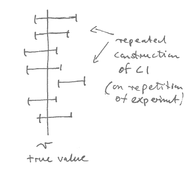
• Note that a CI is actually an estimate: \(\widehat{\text{CI}}(x_1, \ldots, x_n)\), i.e. it depends on data and has a random (sampling) variation.
  
• A good CI has high coverage and is compact.

Note: the coverage probability is not the probability that the true value is contained in a given estimated interval (that would be the Bayesian credible interval).

A.7.9 Symmetric normal confidence interval

For a normally distributed univariate random variable it is straightforward to construct a symmetric two-sided CI with a given desired coverage \(\kappa\).

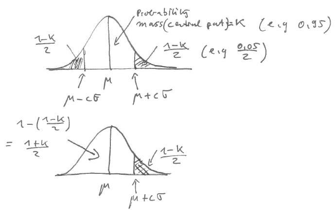
For a normal random variable \(X \sim N(\mu, \sigma^2)\) with mean \(\mu\) and variance \(\sigma^2\) and density function \(f(x)\) we can compute the probability

\[\text{Pr}(x \leq \mu + c \sigma) = \int_{-\infty}^{\mu+c\sigma} f(x) dx = \Phi (c) = \frac{1+\kappa}{2}\] Note \(\Phi(c)\) is the cumulative distribution function (CDF) of the standard normal \(N(0,1)\):

From the above we obtain the critical point \(c\) from the quantile function, i.e. by inversion of \(\Phi\):

\[c=\Phi^{-1}\left(\frac{1+\kappa}{2}\right)\]

The following table lists \(c\) for the three most commonly used values of \(\kappa\) - it is useful to memorise these values!

Coverage \(\kappa\)	Critical value \(c\)
0.9	1.64
0.95	1.96
0.99	2.58

A symmetric standard normal CI with nominal coverage \(\kappa\) for

• a scalar parameter \(\theta\)
• with normally distributed estimate \(\hat{\theta}\) and
• with estimated standard deviation \(\hat{\text{SD}}(\hat{\theta}) = \hat{\sigma}\)

is then given by \[ \widehat{\text{CI}}=[\hat{\theta} \pm c \hat{\sigma}] \] where \(c\) is chosen for desired coverage level \(\kappa\).

A.7.10 Confidence interval based on the chi-squared distribution

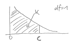
As for the normal CI we can compute critical values but for the chi-squared distribution we use a one-sided interval: \[ \text{Pr}(x \leq c) = \kappa \] As before we get \(c\) by the quantile function, i.e. by inverting the CDF of the chi-squared distribution.

The following list the critical values for the three most common choice of \(\kappa\) for \(m=1\) (one degree of freedom):

Coverage \(\kappa\)	Critical value \(c\) (\(m=1\))
0.9	2.71
0.95	3.84
0.99	6.63

A one-sided CI with nominal coverage \(\kappa\) is then given by \([0, c ]\).