14 Overview over regression modelling
14.1 General setup
\(y\): response variable, also known as outcome or label
\(x_1, x_2, x_3, \ldots, x_d\): predictor variables, also known as covariates or covariables
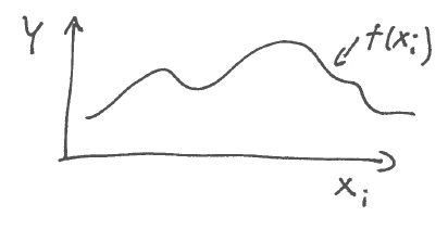
The relationship between the outcomes and the predictor variables is assumed to follow \[ y = f(x_1,x_2,\dots,x_d) + \varepsilon \] where \(f\) is the regression function (not a density) and \(\varepsilon\) represents noise.
14.2 Objectives
Understand the relationship between the response \(y\) and the predictor variables \(x_i\) by learning the regression function \(f\) from observed data (training data). The estimated regression function is \(\hat{f}\).
-
Prediction of outcomes \[\underbrace{\hat{y}}_{\substack{\text{predicted response} \\ \text{using fitted $\hat{f}$}}} = \hat{f}(x_1,x_2,\dots,x_d)\]
If instead of the fitted function \(\hat{f}\) the known regression function \(f\) is used we denote this by \[\underbrace{y^{\star}}_{\substack{\text{predicted response} \\ \text{using known $f$}}} = f(x_1,x_2,\dots,x_d) \]
-
Variable importance
- which covariates are most relevant in predicting the outcome?
- allows to better understand the data and model
\(\rightarrow\) variable selection (to build simpler model with same predictive capability)
14.3 Regression as a form of supervised learning
Regression modelling is a special case of supervised learning.
In supervised learning we make use of labelled data, i.e. \(\boldsymbol x_i\) has an associated label \(y_i\). Thus, the data is consists of pairs \((\boldsymbol x_1, y_1),(\boldsymbol x_2 ,y_2),\dots,(\boldsymbol x_n ,y_n)\).
The supervision part of in supervised learning refers to the fact that the labels are given.
In regression typically the label \(y_i\) is continuous and called the response.
On the other hand, if the label \(y_i\) is discrete/categorical then supervised learning is called classification.
\[\begin{align*} \begin{array}{ll} \\ \text{Supervised Learning}\\ \\ \end{array} \begin{array}{ll} \longrightarrow \text{Discrete } y\\ \\ \longrightarrow \text{Continuous } y\\ \end{array} \begin{array}{ll} \longrightarrow \text{Classification Methods}\\ \\ \longrightarrow \text{Regression Methods}\\ \end{array} \end{align*}\]
Another important type of statistical learning is unsupervised learning where labels \(y\) are inferred from the data \(\boldsymbol x\) (this is also known as clustering). Furthermore, there is also semi-supervised learning with labels only partly known.
Note that there are regression models (e.g. logistic regression) with discrete response that are performing classification, so one may argue that “supervised learning”=“generalised regression”.
14.4 Various regression models used in statistics
In this course we only study linear multiple regression. However, you should be aware that the linear model is in fact just a special cases of some much more general regression approaches.
General regression model: \[y = f(x_1,\dots,x_d) + \text{"noise"}\]
The function \(f\) is estimated nonparametrically - splines - Gaussian processes
Generalised Additive Models (GAM): - the function \(f\) is assumed to be the sum of individual functions \(f_i(x_i)\)
Generalised Linear Models (GLM): - \(f\) is a transformed linear predictor \(h(\sum b_i x_i)\), noise is assumed from an exponential family
Linear Model (LM): - linear predictor \(\sum b_i x_i\), normal noise
In R the linear model is implemented in the function lm(), and generalised linear models in the function glm(). Generalised additive models are available in the package “mgcv”.
In the following we focus on the linear regression model with continuous response.