B Distributions used in Bayesian analysis

This appendix introduces a number of distributions essential for Bayesian analysis.

See in particular the Chapter “Bayesian learning in practise”.

B.1 Beta distribution

B.1.1 Standard parameterisation

The density of the beta distribution \(\text{Beta}(\alpha, \beta)\) is \[ p(x | \alpha, \beta) = \frac{1}{B(\alpha, \beta)} x^{\alpha-1} (1-x)^{\beta-1} \] with \(x \in [0,1]\) and \(\alpha>0\) and \(\beta>0\). The density depends on the beta function \(B(z_1, z_1) = \frac{ \Gamma(z_1) \Gamma(z_2)}{\Gamma(z_1 + z_2)}\) which in turn is defined via Euler’s gamma function \(\Gamma(x)\). Note that \(\Gamma(x) = (x-1)!\) for any positive integer \(x\).

The mean of the beta distribution is \[ \text{E}(x) = \frac{\alpha}{\alpha+\beta} \] and its variance is \[ \text{Var}(x)=\frac{\alpha \beta}{(\alpha+\beta)^2 (\alpha+\beta+1)} \]

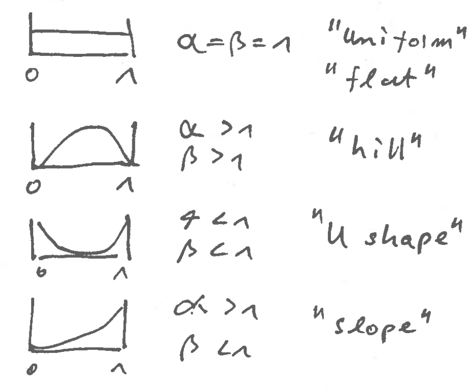
The beta distribution is very flexible and can assume a number of different shapes, depending on the value of \(\alpha\) and \(\beta\):

B.1.2 Mean parameterisation

A useful reparameterisation \(\text{Beta}(\mu, k)\) of the beta distribution is in terms of a mean parameter \(\mu \in [0,1]\) and a concentration parameter \(k > 0\). These are given by \[ k=\alpha+\beta \] and \[\mu = \frac{\alpha}{\alpha+\beta} \] The original parameters can be recovered by \[\alpha= \mu k\] and \[\beta=(1-\mu) k\]

The mean and variance of the beta distribution expressed in terms of \(\mu\) and \(k\) are \[ \text{E}(x) = \mu \] and \[ \text{Var}(x)=\frac{\mu (1-\mu)}{k+1} \] With increasing concentration parameter \(k\) the variance decreases and thus the probability mass becomes more concentrated around the mean.

B.2 Inverse gamma (inverse Wishart) distribution

B.2.1 Standard parameterisation

The inverse gamma (IG) distribution \(\text{Inv-Gam}(\alpha, \beta)\) has density \[ \frac{\beta^{\alpha}}{\Gamma(\alpha)} (1/x)^{\alpha+1} e^{-\beta/x} \] with two parameters \(\alpha >0\) (shape parameter) and \(\beta >0\) (scale parameter) and support \(x >0\).

The mean of the inverse gamma distribution is \[\text{E}(x) = \frac{\beta}{\alpha-1}\] and the variance \[\text{Var}(x) = \frac{\beta^2}{(\alpha-1)^2 (\alpha-2)}\]

Thus, for the mean to exist we have the restriction \(\alpha>1\) and for the variance to exist \(\alpha>2\).

The IG distribution is closely linked with the gamma distribution. If \(x \sim \text{Inv-Gam}(\alpha, \beta)\) is IG-distributed then the inverse of \(x\) is gamma distributed: \[\frac{1}{x} \sim \text{Gam}(\alpha, \theta=\beta^{-1})\] where \(\alpha\) is the shared shape parameter and \(\theta\) the scale parameter of the gamma distribution.

B.2.2 Wishart parameterisation

The inverse gamma distribution is frequently used with a different set of parameters \(\psi = 2\beta\) (scale parameter) and \(\nu = 2\alpha\) (shape parameter), or conversely \(\alpha=\nu/2\) and \(\beta=\psi/2\). In this form it is called one-dimensional inverse Wishart distribution \(W^{-1}_1(\psi, \nu)\) with mean and variance given by \[ \text{E}(x) = \frac{\psi}{\nu-2} = \mu \] for \(\nu>2\) and \[ \text{Var}(x) =\frac{2 \psi^2}{(\nu-4) (\nu-2)^2} = \frac{2 \mu^2}{\nu-4} \] for \(\nu >4\).

Instead of \(\psi\) and \(\nu\) we may also equivalently use \(\mu\) and \(\kappa=\nu-2\) as parameters for the inverse Wishart distribution, so that \(W^{-1}_1(\psi=\kappa \mu, \nu=\kappa+2)\) has mean \[\text{E}(x) = \mu\] with \(\kappa>0\) and the variance is \[\text{Var}(x) = \frac{2 \mu^2}{\kappa-2}\] with \(\kappa>2\). This mean parameterisation is useful when employing the IG distribution as prior and posterior.

Finally, with \(W^{-1}_1(\psi=\nu \tau^2, \nu)\), where \(\tau^2 = \mu \frac{ \kappa}{\kappa+2} = \frac{\psi}{\nu}\) is a biased mean parameter, we get the scaled inverse chi-squared distribution \(\tau^2 \text{Inv-$\chi^2_{\nu}$}\) with \[ \text{E}(x) = \tau^2 \frac{ \nu}{\nu-2} \] for \(\nu>2\) and \[ \text{Var}(x) =\frac{2 \tau^4}{\nu-4} \frac{\nu^2}{(\nu-2)^2} \] for \(\nu >4\).

The inverse Wishart and Wishart distributions are linked. If \(x \sim W^{-1}_1(\psi, \nu)\) is inverse-Wishart distributed then the inverse of \(x\) is Wishart distributed with inverted scale parameter: \[\frac{1}{x} \sim W_1(s^2=\psi^{-1}, k=\nu)\] where \(k\) is the shape parameter and \(s^2\) the scale parameter of the Wishart distribution.

B.3 Location-scale \(t\)-distribution as compound distribution

Suppose that \[ x | s^2 \sim N(\mu,s^2) \] with corresponding density \(p(x | s^2)\) and mean \(\text{E}(x | s^2) = \mu\) and variance \(\text{Var}(x|s^2) = s^2\).

Now let the variance \(s^2\) be distributed as inverse gamma / inverse Wishart \[ s^2 \sim W^{-1}(\psi=\kappa \sigma^2, \nu=\kappa+2) = W^{-1}(\psi=\tau^2\nu, \nu) \] with corresponding density \(p(s^2)\) and mean \(\text{E}(s^2) = \sigma^2 = \tau^2 \nu/(\nu-2)\). Note we use here both the mean parameterisation (\(\sigma^2, \kappa\)) and the inverse chi-squared parameterisation (\(\tau^2, \nu\)).

The joint density for \(x\) and \(s^2\) is \(p(x, s^2) = p(x | s^2) p(s^2)\). We are interested in the marginal density for \(x\): \[ p(x) = \int p(x, s^2) ds^2 = \int p(s^2) p(x | s^2) ds^2 \] This is a compound distribution of a normal with fixed mean \(\mu\) and variance \(s^2\) varying according the inverse gamma distribution. Calculating the integral results in the location-scale \(t\)-distribution with parameters \[ x \sim \text{lst}\left(\mu, \sigma^2 \frac{\kappa}{\kappa+2}, \kappa+2\right) = \text{lst}\left(\mu, \tau^2, \nu\right) \] with mean \[ \text{E}(x) = \mu \] and variance \[ \text{Var}(x) = \sigma^2 =\tau^2 \frac{\nu}{\nu-2} \]

From the law of total expectation and variance we can also directly verify that \[ \text{E}(x) = \text{E}( \text{E}(x| s^2) ) =\mu \] and \[ \text{Var}(x) = \text{E}(\text{Var}(x|s^2))+ \text{Var}(\text{E}(x|s^2)) = \text{E}(s^2) = \sigma^2 =\tau^2 \frac{\nu}{\nu-2} \]