9 Essentials of Bayesian statistics
9.1 Principle of Bayesian learning
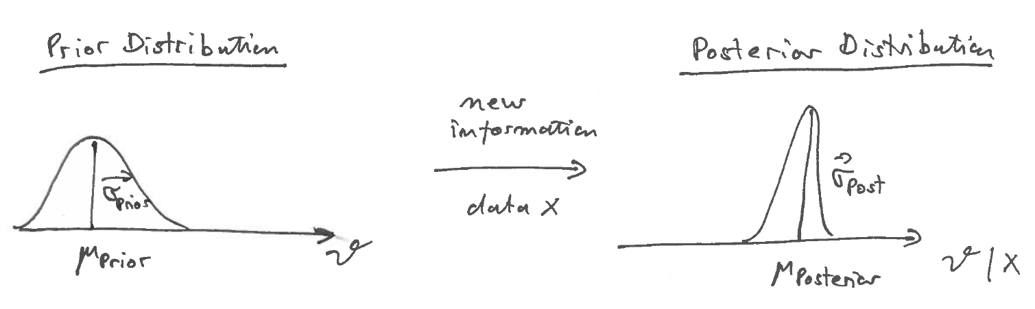
9.1.1 From prior to posterior distribution
Bayesian statistical learning applies Bayes’ theorem to update our state of knowledge about a parameter in the light of data.
Ingredients:
- \(\boldsymbol \theta\) parameter(s) of interest, unknown and fixed.
- prior distribution with density \(p(\boldsymbol \theta)\) describing the uncertainty (not randomness!) about \(\boldsymbol \theta\)
- data generating process \(p(x | \boldsymbol \theta)\)
Note the model underlying the Bayesian approach is the joint distribution \[ p(\boldsymbol \theta, x) = p(\boldsymbol \theta) p(x | \boldsymbol \theta) \] as both a prior distribution over the parameters as well as a data generating process have to be specified.
Question: new information in the form of new observation \(x\) arrives - how does the uncertainty about \(\boldsymbol \theta\) change?
Answer: use Bayes’ theorem to update the prior density to the posterior density.
\[ \underbrace{p(\boldsymbol \theta| x)}_{\text{posterior} } = \underbrace{p(\boldsymbol \theta)}_{\text{prior}} \frac{p(x | \boldsymbol \theta) }{ p(x)} \]
For the denominator in Bayes formula we need to compute \(p(x)\).
This is obtained by
\[
\begin{split}
p(x) &= \int_{\boldsymbol \theta} p(x , \boldsymbol \theta) d\boldsymbol \theta\\
&= \int_{\boldsymbol \theta} p(x | \boldsymbol \theta) p(\boldsymbol \theta) d\boldsymbol \theta\\
\end{split}
\]
i.e. by marginalisation of the parameter \(\boldsymbol \theta\) from the joint
distribution of \(\boldsymbol \theta\) and \(x\).
(For discrete \(\boldsymbol \theta\) replace the integral by a sum).
Depending on the context this quantity is either called the
- normalisation constant as it ensures that the posterior density \(p(\boldsymbol \theta| x)\) integrates to one.
- prior predictive density of the data \(x\) given the model \(M\) before seeing any data. To emphasise the implicit conditioning on a model we may write \(p(x| M)\). Since all parameters have been integrated out \(M\) in fact refers to a model class.
- marginal likelihood of the underlying model (class) \(M\) given data \(x\). To emphasise this may write \(L(M| x)\). Sometimes it is also called model likelihood.
9.1.2 Zero forcing property
It is easy to see that if in Bayes rule the prior density/probability is zero for some parameter value \(\boldsymbol \theta\) then the posterior density/probability will remain at zero for that \(\boldsymbol \theta\), regardless of any data collected. This zero-forcing property of the Bayes update rule has been called Cromwell’s rule by Dennis Lindley (1923–2013). Therefore, assigning prior density/probability 0 to an event should be avoided.
Note that this implies that assigning prior probability 1 should be avoided, too.
9.1.3 Bayesian update and likelihood
After independent and identically distributed data \(D = \{x_1, \ldots, x_n\}\) have been observed the Bayesian posterior is computed by
\[
\underbrace{p(\boldsymbol \theta| D) }_{\text{posterior} } = \underbrace{p(\boldsymbol \theta)}_{\text{prior}} \frac{ L(\boldsymbol \theta| D) }{ p(D)}
\]
involving the likelihood \(L(\boldsymbol \theta| D) = \prod_{i=1}^n p(x_i | \boldsymbol \theta)\)
and the marginal likelihoood \(p(D) = \int_{\boldsymbol \theta} p(\boldsymbol \theta) L(\boldsymbol \theta| D) d\boldsymbol \theta\) with \(\boldsymbol \theta\) integrated out.
The marginal likelihood serves as a standardising factor so that the posterior density for \(\boldsymbol \theta\) integrates to 1: \[ \int_{\boldsymbol \theta} p(\boldsymbol \theta| D) d\boldsymbol \theta= \frac{1}{p(D)} \int_{\boldsymbol \theta} p(\boldsymbol \theta) L(\boldsymbol \theta| D) d\boldsymbol \theta= 1 \] Unfortunately, the integral to compute the marginal likelihood is typically analytically intractable and requires numerical integration and/or approximation.
Comparing likelihood and Bayes procedures note that
- conducting a Bayesian statistical analysis requires integration respectively averaging (to compute the marginal likelihood)
- in contrast to a likelihood analysis that requires optimisation (to find the maximum likelihood).
9.1.4 Sequential updates
Note that the Bayesian update procedure can be repeated again and again: we can use the posterior as our new prior and then update it with further data. Thus, we may also update the posterior density sequentially, with the data points \(x_1, \ldots, x_n\) arriving one after the other, by computing first \(p(\boldsymbol \theta| x_1)\), then \(p(\boldsymbol \theta| x_1, x_2)\) and so on until we reach \(p(\boldsymbol \theta| x_1, \ldots, x_n) = p(\boldsymbol \theta| D)\).
For example, for the first update we have \[ p(\boldsymbol \theta| x_1) = p(\boldsymbol \theta) \frac{p(x_1 | \boldsymbol \theta) }{p(x_1)} \] with \(p(x_1) =\int_{\boldsymbol \theta} p(x_1 | \boldsymbol \theta) p(\boldsymbol \theta) d\boldsymbol \theta\). The second update yields \[ \begin{split} p(\boldsymbol \theta| x_1, x_2) &= p(\boldsymbol \theta| x_1) \frac{p(x_2 | \boldsymbol \theta, x_1) }{p(x_2| x_1)}\\ &= p(\boldsymbol \theta| x_1) \frac{p(x_2 | \boldsymbol \theta) }{p(x_2| x_1)}\\ &= p(\boldsymbol \theta) \frac{ p(x_1 | \boldsymbol \theta) p(x_2 | \boldsymbol \theta) }{p(x_1) p(x_2| x_1)}\\ \end{split} \] with \(p(x_2| x_1) = \int_{\boldsymbol \theta} p(x_2 | \boldsymbol \theta) p(\boldsymbol \theta| x_1) d\boldsymbol \theta\). The final step is \[ \begin{split} p(\boldsymbol \theta| D) = p(\boldsymbol \theta| x_1, \ldots, x_n) &= p(\boldsymbol \theta) \frac{ \prod_{i=1}^n p(x_i | \boldsymbol \theta) }{ p(D) }\\ \end{split} \] with the marginal likelihood factorising into \[ p(D) = \prod_{i=1}^n p(x_i| x_{<i}) \] with \[ p(x_i| x_{<i}) = \int_{\boldsymbol \theta} p(x_i | \boldsymbol \theta) p(\boldsymbol \theta| x_{<i}) d\boldsymbol \theta \] The last factor is the posterior predictive density of the new data \(x_i\) after seeing data \(x_1, \ldots, x_{i-1}\) (given the model class \(M\)). It is straightforward to understand why the probability of the new \(x_i\) depends on the previously observed data points — because the uncertainty about the model parameter \(\boldsymbol \theta\) depends on how much data we have already observed. Therefore the marginal likelihood \(p(D)\) is not simply the product of the marginal densities \(p(x_i)\) at each \(x_i\) but instead the product of the conditional densities \(p(x_i| x_{<i})\).
Only when the parameter is fully known and there is no uncertainty about \(\boldsymbol \theta\) the observations \(x_i\) are independent. This leads back to the standard likelihood where we condition on a particular \(\boldsymbol \theta\) and the likelihood is the product \(p(D| \boldsymbol \theta) = \prod_{i=1}^n p(x_i| \boldsymbol \theta)\).
9.1.5 Summaries of posterior distributions and credible intervals
The Bayesian estimate is the full complete posterior distribution!
However, it is useful to summarise aspects of the posterior distribution:
- Posterior mean \(\text{E}(\boldsymbol \theta| D)\)
- Posterior variance \(\text{Var}(\boldsymbol \theta| D)\)
- Posterior mode etc.
In particular the mean of the posterior distribution is often taken as a Bayesian point estimate.
The posterior distribution also allows to define credible regions or credible intervals. These are the Bayesian equivalent to confidence intervals and are constructed by finding the areas of highest probability mass (say 95%) in the posterior distribution.
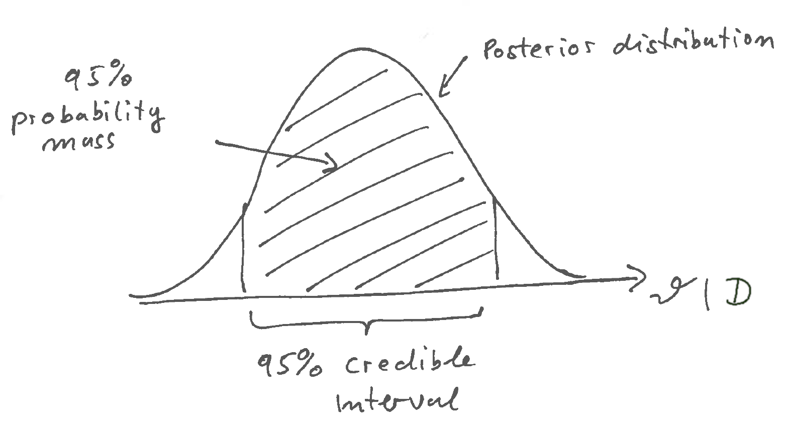
Bayesian credible intervals (unlike their frequentist confidence counterparts) are thus very easy to interpret - they simply correspond to the area in the parameter space in which the we can find the parameter with a given specified probability. In contrast, in frequentist statistics it does not make sense to assign a probability to a parameter value!
Note that there are typically many credible intervals with the given specified coverage \(\alpha\) (say 95%). Therefore, we may need further criteria to construct these intervals.
For univariate parameter \(\theta\) a two-sided equal-tail credible interval is obtained by finding the corresponding lower \(1-\alpha/2\) and upper \(\alpha/2\) quantiles. Typically this type of credible interval is easy to compute. However, note that the density values at the left and right boundary points of such an interval are typically different. Also this does not generalise well to a multivariate parameter \(\boldsymbol \theta\).
As alternative, a highest posterior density (HPD) credible interval of coverage \(\alpha\) is found by identifying the shortest interval (i.e. with smallest support) for the given \(\alpha\) probability mass. Any point within an HDP credible interval has higher density than a point outside the HDP credible interval. Correspondingly, the density at the boundary of an HPD credible interval is constant taking on the same value everywhere along the boundary.
A Bayesian HPD credible interval is constructed in a similar fashion as a likelihood-based confidence interval, starting from the mode of the posterior density and then looking for a common threshold value for the density to define the boundary of the credible interval. When the posterior density has multiple modes the HPD interval may be disjoint. HPD intervals are also well defined for multivariate \(\boldsymbol \theta\) with the boundaries given by the contour lines of the posterior density resulting from the threshold value.
In the Worksheet B1 examples for both types of credible intervals are given and compared visually.
9.1.6 Practical application of Bayes statistics on the computer
As we have seen Bayesian learning is conceptually straightforward:
- Specify prior uncertainty \(p(\boldsymbol \theta\)) about the parameters of interest \(\boldsymbol \theta\).
- Specify the data generating process for a specified parameter: \(p(x | \boldsymbol \theta)\).
- Apply Bayes’ theorem to update prior uncertainty in the light of the new data.
In practise, however, computing the posterior distribution can be computationally very demanding, especially for complex models.
For this reason specialised software packages have been developed for computational Bayesian modelling, for example:
Bayesian statistics in R: https://cran.r-project.org/web/views/Bayesian.html
Stan probabilistic programming language (interfaces with R, Python, Julia and other languages) — https://mc-stan.org/
Bayesian statistics in Python: PyMC using Aesara/JAX as backend, NumPyro using JAX as backend, TensorFlow Probability on JAX using JAX as backend, PyMC3 using Theano as backend, Pyro using PyTorch as backend, TensorFlow Probability using Tensorflow as backend.
Bayesian statistics in Julia: Turing.jl
In addition to numerical procedures to sample from the posterior distribution there are also many procedures aiming to approximate the Bayesian posterior, employing the Laplace approximation, integrated nested Laplace approximation (INLA), variational Bayes etc.
9.2 Some background on Bayesian statistics
9.2.1 Bayesian interpretation of probability
9.2.1.1 What makes you “Bayesian”?
If you use Bayes’ theorem are you therefore automatically a Bayesian? No!!
Bayes’ theorem is a mathematical fact from probability theory. Hence, Bayes’ theorem is valid for everyone, whichever form for statistical learning your are subscribing (such as frequentist ideas, likelihood methods, entropy learning, Bayesian learning).
As we discuss now the key difference between Bayesian and frequentist statistical learning lies in the differences in interpretation of probability, not in the mathematical formalism for probability (which includes Bayes’ theorem).
9.2.1.2 Mathematics of probability
The mathematics of probability in its modern foundation was developed by Andrey Kolmogorov (1903–1987). In this book Foundations of the Theory of Probability (1933) he establishes probability in terms of set theory/ measure theory. This theory provides a coherent mathematical framework to work with probabilities.
However, Kolmogorov’s theory does not provide an interpretation of probability!
\(\rightarrow\) The Kolmogorov framework is the basis for both the frequentist and the Bayesian interpretation of probability.
9.2.1.3 Interpretations of probability
Essentially, there are two major commonly used interpretation of probability in statistics - the frequentist interpretation and the Bayesian interpretation.
A: Frequentist interpretation
probability = frequency (of an event in a long-running series of identically repeated experiments)
This is the ontological view of probability (i.e. probability “exists” and is identical to something that can be observed.).
It is also a very restrictive view of probability. For example, frequentist probability cannot be used to describe events that occur only a single time. Frequentist probability thus can only be applied asymptotically, for large samples!
B: Bayesian probability
“Probability does not exist” — famous quote by Bruno de Finetti (1906–1985), a Bayesian statistician.
What does this mean?
Probability is a description of the state of knowledge and of uncertainty.
Probability is thus an epistemological quantity that is assigned and that changes rather than something that is an inherent property of an object.
Note that this does not require any repeated experiments. The Bayesian interpretation of probability is valid regardless of sample size or the number or repetitions of an experiment.
Hence, the key difference between frequentist and Bayesian approaches is not the use of Bayes’ theorem. Rather it is whether you consider probability as ontological (frequentist) or epistemological entity (Bayesian).
9.2.2 Historical developments
- Bayesian statistics is named after Thomas Bayes (1701-1761). His paper 8 introducing the famous theorem was published only after his death (1763).
- Pierre-Simon Laplace (1749-1827) was the first to practically use Bayes’ theorem for statistical calculations, and he also independently discovered Bayes’ theorem in 1774 9
This activity was then called “inverse probability” and not “Bayesian statistics”.
Between 1900 and 1940 classical mathematical statistics was developed and the field was heavily influenced and dominated by R.A. Fisher (who invented likelihood theory and ANOVA, among other things - he was also working in biology and was professor of genetics). Fisher was very much opposed to Bayesian statistics.
1931 Bruno de Finetti publishes his “representation theorem”. This shows that the joint distribution of a sequence of exchangeable events (i.e. where the ordering can be permuted) can be represented by a mixture distribution that can be constructed via Bayes’ theorem. (Note that exchangeability is a weaker condition than i.i.d.) This theorem is often used as a justification of Bayesian statistics (along with the so-called Dutch book argument, also by de Finetti).
1933 publication of Andrey Kolmogorov’s book on probability theory.
1946 Cox theorem by Richard T. Cox (1898–1991): the aim to generalise classical logic from TRUE/FALSE statements to continuous measures of uncertainty inevitably leads to probability theory and Bayesian learning! This justification of Bayesian statistics was later popularised by Edwin T. Jaynes (1922–1998) in various books (1959, 2003).
1955 Stein Paradox - Charles M. Stein (1920–2016) publishes a paper on the Stein estimator — an estimator of the mean that dominates the ML estimator (i.e. the sample average). The Stein estimator is better in terms of MSE than the ML estimator, which was very puzzling at that time but it is easy to understand from a Bayesian perspective.
Only from the 1950s the use of the term “Bayesian statistics” became prevalent — see Fienberg (2006) 10
Due to advances in personal computing from 1970 onwards Bayesian learning has become more pervasive!
- Computers allow to do the complex (numerical) calculations needed in Bayesian statistics .
- Metropolis-Hastings algorithm published in 1970 (which allows to sample from a posterior distribution without explicitly computing the marginal likelihood).
- Development of regularised estimation techniques such as penalised likelihood in regression (e.g. ridge regression 1970).
- penalised likelihood via KL divergence for model selection (Akaike 1973).
- A lot of work on interpreting Stein estimators as empirical Bayes estimators (Efron and Morris 1975)
- regularisation originally was only meant to make singular systems/matrices invertible, but then it turned out regularisation has also a Bayesian interpretation.
- Reference priors (Bernardo 1979) proposed as default priors for models with multiple parameters.
- The EM algorithm (published in 1977) uses Bayes theorem for imputing the distribution of the latent variables.
Another boost was in the 1990/2000s when in science (e.g. genomics) many complex and high-dimensional data set were becoming the norm, not the exception.
- Classical statistical methods cannot be used in this setting (overfitting!) so new methods were developed for high-dimensional data analysis, many with a direct link to Bayesian statistics
- 1996 lasso (L1 regularised) regression invented by Robert Tibshirani.
- Machine learning methods for non-parametric and extremely highly parametric models (neural network) require either explicit or implicit regularisation.
- Many Bayesians in this field, many using variational Bayes techniques which may be viewed as generalisation of the EM algorithm and are also linked to methods used in statistical physics.