9 Observed Fisher information
9.1 Definition of the observed Fisher information
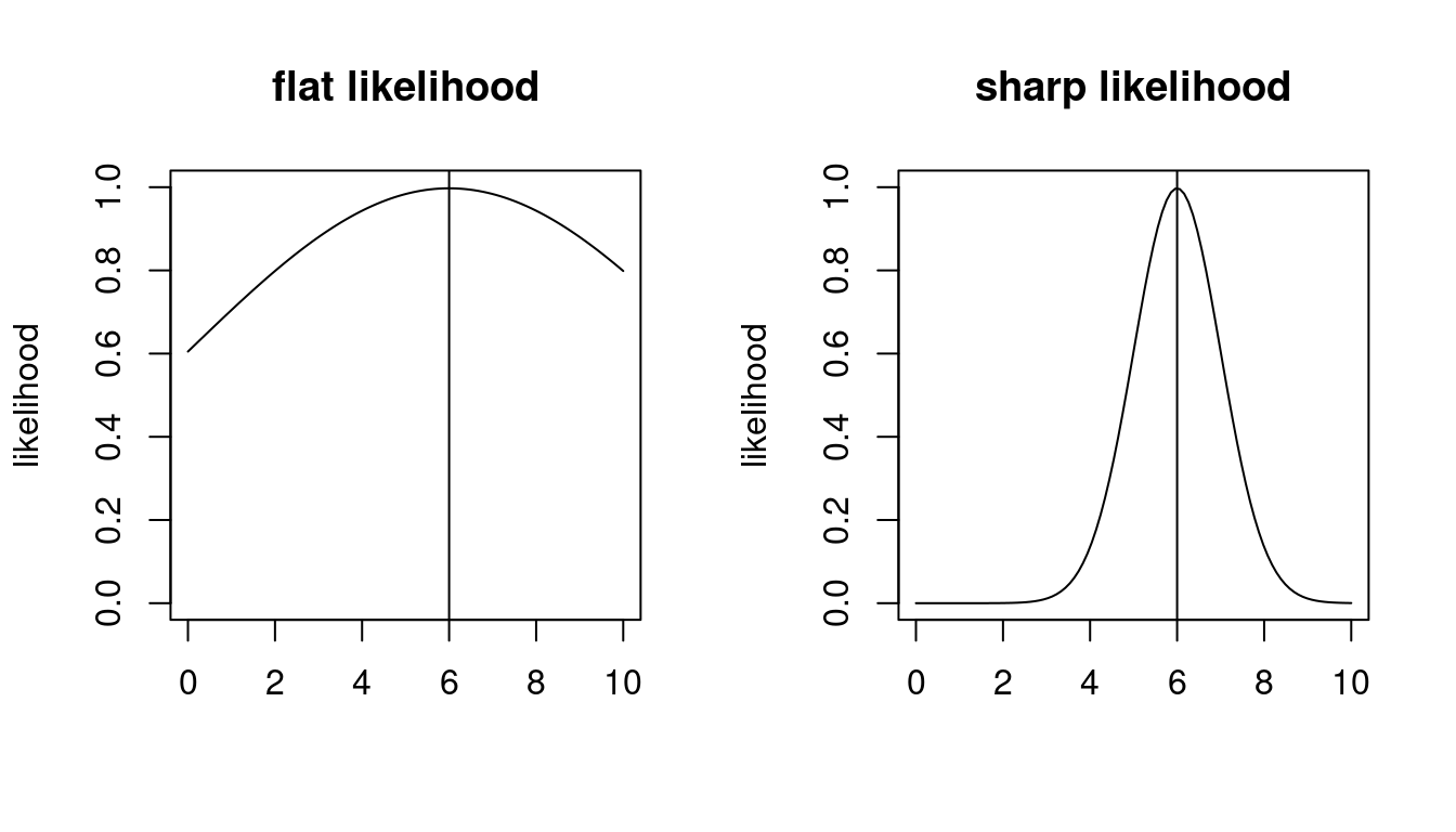
Visual inspection of the log-likelihood function (e.g. Figure 9.1) suggests that it contains more information about the parameter \(\boldsymbol \theta\) than just the location of its maximum at \(\hat{\boldsymbol \theta}_{ML}\).
In particular, in a regular model the curvature of the log-likelihood function at the MLE is linked to the accuracy of \(\hat{\boldsymbol \theta}_{ML}\): a flat log-likelihood surface near the maximum (low curvature) makes the optimal parameter less well determined (and more difficult find numerically). Conversely, if the log-likelihood surface is sharply peaked (strong curvature) then the maximum point is well defined. The curvature can be quantified by the matrix of second-order derivatives (Hessian matrix) of the log-likelihood function.
Accordingly, the observed Fisher information (matrix) is defined as the negative Hessian of the log-likelihood function \(\ell_n(\boldsymbol \theta)\) at the MLE \(\hat{\boldsymbol \theta}_{ML}\): \[ {\boldsymbol J_n}(\hat{\boldsymbol \theta}_{ML}) = -\nabla \nabla^T \ell_n(\hat{\boldsymbol \theta}_{ML}) \] With \(\ell_n ({\boldsymbol \theta}) = n \operatorname{E}_{\hat{Q}_n}(\log p(x | \boldsymbol \theta))\) we can also write it as \[ \begin{split} {\boldsymbol J_n}(\hat{\boldsymbol \theta}_{ML}) &= - n \operatorname{E}_{\hat{Q}_n} \left( \nabla \nabla^T \log p(x | \hat{\boldsymbol \theta}_{ML} ) \right) \\ &= n \boldsymbol J_P( \hat{\boldsymbol \theta}_{ML}) \end{split} \] with \[ \boldsymbol J_P( \boldsymbol \theta) = -\operatorname{E}_{ \hat{Q}_n } \left( \nabla \nabla^T \log p(x|\boldsymbol \theta)\right) \]
To avoid confusion with the Fisher information \[ \boldsymbol{\mathcal{I}}_{P}(\boldsymbol \theta) = -\operatorname{E}_{P(\boldsymbol \theta)} \left( \nabla \nabla^T \log p(x|\boldsymbol \theta)\right) \] introduced earlier (Section 5.1) it is necessary to always use the qualifier “observed” when referring to \({\boldsymbol J_n}(\hat{\boldsymbol \theta}_{ML})\).
The observed Fisher information plays an important role in quantifying the uncertainty of a maximum likelihood estimate.
Transformation properties
As a consequence of the invariance of the score function and curvature function the observed Fisher information is invariant under transformations of the sample space. This is the same invariance also shown by the Fisher information and by the KL divergence.
\(\color{Red} \blacktriangleright\) Like the Fisher information the observed Fisher information (as a Hessian matrix) transforms covariantly under change of model parameters — see Section 5.2.1.
Relationship between observed and expected Fisher information
The observed Fisher information \(\boldsymbol J_n(\hat{\boldsymbol \theta}_{ML})\) and the expected Fisher information \(\boldsymbol{\mathcal{I}}_{P}(\boldsymbol \theta)\) are related but also two clearly different entities.
Curvature based:
- Both types of Fisher information are based on computing second order derivatives (Hessian matrix), thus both are based on the curvature of a function.
Transformation properties:
Both quantities are invariant under changes of the parametrisation of the sample space.
\(\color{Red} \blacktriangleright\) Both transform covariantly when changing the parameter of the distribution.
Data-based vs. model only:
The observed Fisher information is computed from the log-likelihood function. Therefore it takes both the model and the observed data \(D\) into account and explicitly depends on the sample size \(n\). It contains estimates of the parameters but not the parameters themselves. While the curvature of the log-likelihood function may be computed for any point of the log-likelihood function the observed Fisher information specifically refers to the curvature at the MLE \(\hat{\boldsymbol \theta}_{ML}\). It is linked to the (asymptotic) variance of the MLE (see the examples and as will be discussed in more detail later).
In contrast, the expected Fisher information is derived directly from the log-density of the model family. It does not depend on the observed data, and thus does not depend on sample size. It is a property of the model family \(P(\boldsymbol \theta)\) alone. It makes sense and can be computed at any \(\boldsymbol \theta\). It describes the local geometry of the space of the model family, and is the local approximation of KL information.
Large sample equivalence for correctly specified models:
- Assume a that \(P(\boldsymbol \theta)\) is correctly specified and that for large sample size \(n\) the MLE converges to \(\hat{\boldsymbol \theta}_{ML} \rightarrow \boldsymbol \theta_{\text{true}}\). It follows from the construction of the observed Fisher information and the law of large numbers that it converges to the Fisher information for a set of iid random variables, see Section 5.1.3. Specifically, \(\boldsymbol J_n(\hat{\boldsymbol \theta}_{ML}) = n \boldsymbol J_P(\hat{\boldsymbol \theta}_{ML}) \rightarrow n \boldsymbol{\mathcal{I}}_{P}( \boldsymbol \theta_{\text{true}} )\)
\(\color{Red} \blacktriangleright\) Finite sample equivalence for exponential families:
In the important class of exponential families the relationship \(\boldsymbol J_n(\hat{\boldsymbol \theta}_{ML}) = n \boldsymbol J_P( \hat{\boldsymbol \theta}_{ML} ) = n \boldsymbol{\mathcal{I}}_{P}( \hat{\boldsymbol \theta}_{ML} )\) is valid also for finite sample size \(n\). The general case is shown in Example 5.5 and Example 9.5 (canonical parameter) and Example 5.8 and Example 9.6 (expectation parameter).
This can also be directly seen from special instances of exponential families such as the Bernoulli distribution (Example 5.1 and Example 9.1), the normal distribution with one parameter (Example 5.3 and Example 9.2) and the normal distribution with two parameters (Example 5.4 and Example 9.4).
- However, exponential families are an exception. In a general model \(\boldsymbol J_n(\hat{\boldsymbol \theta}_{ML}) = \boldsymbol J_P(\hat{\boldsymbol \theta}_{ML}) \neq n \boldsymbol{\mathcal{I}}_{P}( \hat{\boldsymbol \theta}_{ML} )\) for finite sample size \(n\) even when the model \(P(\boldsymbol \theta)\) is correctly specified. As an example consider the location-scale \(t\)-distribution \(t_{\nu}(\mu, \tau^2)\) with unknown median parameter \(\mu\) and known scale parameter \(\tau^2\) and given degree of freedom \(\nu\). This is not an exponential family model (unless \(\nu \rightarrow \infty\) when it becomes the normal distribution). It can be shown that the Fisher information is \(\mathcal{I}_{P}(\mu )=\frac{\nu+1}{\nu+3} \frac{1}{\tau^2}\) but the observed Fisher information \(J_n(\hat{\mu}_{ML}) \neq n \frac{\nu+1}{\nu+3} \frac{1}{\tau^2}\) with a maximum likelihood estimate \(\hat{\mu}_{ML}\) that can only be computed numerically with no closed form available.
9.2 Observed Fisher information examples
Scalar examples — single parameter models
Example 9.1 Observed Fisher information for the Bernoulli model \(\operatorname{Ber}(\theta)\):
We continue Example 8.1. The second derivative of the log-likelihood function is \[ \frac{d s_n(\theta)}{d\theta}=- n \left( \frac{ \bar{x} }{\theta^2} + \frac{1 - \bar{x} }{(1-\theta)^2} \right) \] The observed Fisher information is therefore \[ \begin{split} J_n(\hat{\theta}_{ML}) &= -\frac{d s_n(\hat{\theta}_{ML})}{d\theta} \\ & = n \left(\frac{ \bar{x} }{\hat{\theta}_{ML}^2} + \frac{ 1 - \bar{x} }{ (1-\hat{\theta}_{ML})^2 } \right) \\ & = n \left(\frac{1}{\hat{\theta}_{ML}} + \frac{1}{1-\hat{\theta}_{ML}} \right) \\ &= \frac{n}{\hat{\theta}_{ML} (1-\hat{\theta}_{ML})} \\ \end{split} \]
The inverse of the observed Fisher information is: \[J_n(\hat{\theta}_{ML})^{-1}=\frac{\hat{\theta}_{ML}(1-\hat{\theta}_{ML})}{n}\]
Compare this with \(\operatorname{Var}\left(\frac{x}{n}\right) = \frac{\theta(1-\theta)}{n}\) for \(x \sim \operatorname{Bin}(n, \theta)\).
Example 9.2 Observed Fisher information for the normal distribution with unknown mean and known variance:
This is the continuation of Example 8.2. The second derivative of the log-likelihood function is \[ \frac{d s_n(\mu)}{d\mu}=- \frac{n}{\sigma^2} \] The observed Fisher information at the MLE is therefore \[ J_n(\hat{\mu}_{ML}) = -\frac{d s_n(\hat{\mu}_{ML})}{d\mu} = \frac{n}{\sigma^2} \] and the inverse of the observed Fisher information is \[ J_n(\hat{\mu}_{ML})^{-1} = \frac{\sigma^2}{n} \]
For \(x_i \sim N(\mu, \sigma^2)\) we have \(\operatorname{Var}(x_i) = \sigma^2\) and hence \(\operatorname{Var}(\bar{x}) = \sigma^2/n\), which is equal to the inverse observed Fisher information.
Example 9.3 Observed Fisher information for the normal distribution with known mean and unknown variance:
This is the continuation of Example 8.3. The second derivative of the log-likelihood function is \[ \frac{d s_n(\sigma^2)}{d\sigma^2} = -\frac{n}{2\sigma^4} \left(\frac{2}{\sigma^2} \overline{(x-\mu)^2} -1\right) \] Correspondingly, the observed Fisher information is \[ J_n(\widehat{\sigma^2}_{ML}) = -\frac{d s_n(\widehat{\sigma^2}_{ML})}{d\sigma^2} = \frac{n}{2} \left(\widehat{\sigma^2}_{ML} \right)^{-2} \] and its inverse is \[ J_n(\widehat{\sigma^2}_{ML})^{-1} = \frac{2}{n} \left(\widehat{\sigma^2}_{ML} \right)^{2} \]
With \(x_i \sim N(\mu, \sigma^2)\) the empirical variance \(\widehat{\sigma^2}_{ML}\) follows a one-dimensional Wishart distribution \[ \widehat{\sigma^2}_{\text{ML}} \sim \operatorname{Wis}\left(s^2 = \frac{\sigma^2}{n}, k=n-1\right) \] (see Section A.8) and hence has variance \(\operatorname{Var}(\widehat{\sigma^2}_{ML}) = \frac{n-1}{n} \, \frac{2 \sigma ^4}{n}\). For large \(n\) this becomes \(\operatorname{Var}\left(\widehat{\sigma^2}_{ML}\right)\overset{a}{=} \frac{2}{n} \left(\sigma^2\right)^2\) which is (apart from the “hat”) the inverse of the observed Fisher information.
Matrix examples — multiple parameter models
Example 9.4 Observed Fisher information for the normal distribution with mean and variance parameter:
This is the continuation of Example 8.5.
The Hessian matrix of the log-likelihood function is \[ \begin{split} \nabla \nabla^T \ell_n(\mu,\sigma^2) &= \begin{pmatrix} - \frac{n}{\sigma^2}& -\frac{n}{\sigma^4} (\bar{x} -\mu)\\ - \frac{n}{\sigma^4} (\bar{x} -\mu) & \frac{n}{2\sigma^4}-\frac{n}{\sigma^6} \left(\overline{x^2} - 2 \mu \bar{x} + \mu^2\right) \\ \end{pmatrix} \end{split} \] The negative Hessian at the MLE, i.e. at \(\hat{\mu}_{ML} = \bar{x}\) and \(\widehat{\sigma^2}_{ML} = \overline{x^2} -\bar{x}^2\), yields the observed Fisher information matrix: \[ \begin{split} \boldsymbol J_n(\hat{\mu}_{ML},\widehat{\sigma^2}_{ML}) &= - \nabla \nabla^T \ell_n(\hat{\mu}_{ML},\widehat{\sigma^2}_{ML}) \\ &= \begin{pmatrix} \frac{n}{\widehat{\sigma^2}_{ML}}&0 \\ 0 & \frac{n}{2(\widehat{\sigma^2}_{ML})^2} \end{pmatrix} \end{split} \] The observed Fisher information matrix is diagonal with positive entries. Therefore its eigenvalues are all positive as required for a maximum, because for a diagonal matrix the eigenvalues are the the entries on the diagonal.
The inverse of the observed Fisher information matrix is \[ \boldsymbol J_n(\hat{\mu}_{ML},\widehat{\sigma^2}_{ML})^{-1} = \begin{pmatrix} \frac{\widehat{\sigma^2}_{ML}}{n}& 0\\ 0 & \frac{2(\widehat{\sigma^2}_{ML})^2}{n} \end{pmatrix} \]
Example 9.5 \(\color{Red} \blacktriangleright\) Observed Fisher information for the canonical parameter of an exponential family:
This is the continuation of Example 8.7.
The Hessian matrix of the log-likelihood function is \[ \begin{split} \nabla \nabla^T \ell_n(\boldsymbol \eta) &= -n \nabla \nabla^T a(\boldsymbol \eta)\\ & = -n \boldsymbol \Sigma_{\boldsymbol t}(\boldsymbol \eta)\\ \end{split} \] with \(\operatorname{Var}( \boldsymbol t(x) ) = \boldsymbol \Sigma_{\boldsymbol t}\).
Assuming a minimal exponential family with nonredundant canonical parameters and strictly convex log-partition function \(a(\boldsymbol \eta)\) the covariance matrix \(\boldsymbol \Sigma_{\boldsymbol t}\) will be positive definite and therefore the eigenvalues of the Hessian will all be positive as required for a maximum. Conversely, if the model is nonminimal the Hessian will be singular, i.e. there will be some eigenvalues of value zero indicating that there is dependence among the parameters.
The negative Hessian at the MLE yields the observed Fisher information matrix for the canonical parameter: \[ \boldsymbol J_n(\hat{\boldsymbol \eta}_{ML}) = n \boldsymbol \Sigma_{\boldsymbol t}( \hat{\boldsymbol \eta}_{ML} ) \] Compare with the corresponding expected Fisher information (Example 5.5).
Example 9.6 \(\color{Red} \blacktriangleright\) Observed Fisher information for the expectation parameter of an exponential family:
Instead of the observed Fisher information for the canonical parameter \(\boldsymbol \eta\) we are often rather more interested in the Fisher information for the expectation parameter \(\boldsymbol \mu_{\boldsymbol t}\).
Similarly as for the Fisher information (see Example 5.8) we may transform the observed Fisher information to the expectation parameter via covariant transformation and get \[ \boldsymbol J_n\left(\hat{\boldsymbol \mu}_{\boldsymbol t}^{ML}\right) = n \boldsymbol \Sigma_{\boldsymbol t}\left(\boldsymbol \eta\left(\hat{\boldsymbol \mu}_{\boldsymbol t}^{ML}\right)\right)^{-1} \] The inverse of the observed Fisher information matrix is \[ \boldsymbol J_n\left(\hat{\boldsymbol \mu}_{\boldsymbol t}^{ML}\right)^{-1} = \frac{1}{n} \boldsymbol \Sigma_{\boldsymbol t}\left(\boldsymbol \eta\left(\hat{\boldsymbol \mu}_{\boldsymbol t}^{ML}\right)\right) \]