7  Nonlinear and nonparametric models

In the last part of the module we discuss methods that go beyond the linear parametric methods prevalent in classical multivariate statistics.

Relevant textbooks:

The lectures for much of this part of the module follow selected chapters from the following text books:

• James et al. (2021) An introduction to statistical learning with applications in R (2nd edition). Springer.

• Rogers and Girolami (2017) A first course in machine learning (2nd edition). CRC Press.

Please study the relevant section and chapters as indicated below in each subsection!

The first book is also available in a version whith examples in Python:

• James et al. (2023) An introduction to statistical learning with applications in Python. Springer.

7.1 Random forests

Another widely used approach for prediction in nonlinear settings is the method of random forests.

Relevant reading:

Please read: James et al. (2021) or James et al. (2023) Chapter 8 “Tree-Based Methods”

Specifically:

• Section 8.1 The Basics of Decision Trees
• Section 8.2.1 Bagging
• Section 8.2.2 Random Forests

Stochastic vs. algorithmic models

Two cultures in statistical modelling: stochastic vs. algorithmic models

Classic discussion paper by Leo Breiman (2001): Statistical modeling: the two cultures. Statistical Science 16:199–231. https://doi.org/10.1214/ss/1009213726

This paper has recently be revisited in the following discussion paper by Efron (2020) and discussants: Prediction, estimation, and attribution. JASA 115:636–677. https://doi.org/10.1080/01621459.2020.1762613

Random forests

Proposed by Leo Breimann in 2001 as application of “bagging” (Breiman 1996) to decision trees.

Basic idea:

• A single decision tree is unreliable and unstable (weak predictor/classifier).
• Use boostrap to generate multiple decision trees (=“forest”)
• Average over predictions from all tree (=“bagging”, bootstrap aggregation)

The averaging procedure has the effect of variance stabilisation. Intringuingly, averaging across all decision trees dramatically improves the overall prediction accuracy!

The Random Forests approach is an example of an ensemble method (since it is based on using an “ensemble” of trees).

Variations: boosting, XGBoost ( https://xgboost.ai )

Random forests will be applied in Worksheet 11.

They are computationally expensive but typically perform very well!

Comparison of decision boundaries: decision tree vs. random forest

Figure 7.1: Decision boundaries for decision trees and random forests in the non-nested case.

Figure 7.2: Decision boundaries for decision trees and random forests in the nested case.

Compare the non-nested case (Figure 7.1) and the nested case (Figure 7.2).

Compare also with the decision boundaries for LDA and QDA in Figure 5.4 and Figure 5.5.

7.2 Gaussian processes

Gaussian processes offer a nonparametric probabilistic approach to model nonlinear dependencies.

Relevant reading:

Please read: Rogers and Girolami (2017) Chapter 8: Gaussian processes.

Main concepts

• Gaussian processes (GPs) belong the the family of Bayesian nonparametric models
• Idea:
  • start with prior over a function (!),
  • then condition on observed data to get posterior distribution (again over a function)
• GPs use an infinitely dimensional multivariate normal distribution as prior

Conditional multivariate normal distribution

GPs make use of the fact that marginal and conditional distributions of a multivariate normal distribution are also multivariate normal.

Multivariate normal distribution:

\[\boldsymbol z\sim N_d(\boldsymbol \mu, \boldsymbol \Sigma)\]

Assume: \[ \boldsymbol z=\begin{pmatrix} \boldsymbol z_1 \\ \boldsymbol z_2 \\ \end{pmatrix} \] with \[ \boldsymbol \mu=\begin{pmatrix} \boldsymbol \mu_1 \\ \boldsymbol \mu_2 \\ \end{pmatrix} \] and \[ \boldsymbol \Sigma=\begin{pmatrix} \boldsymbol \Sigma_{1} & \boldsymbol \Sigma_{12} \\ \boldsymbol \Sigma_{12}^T & \boldsymbol \Sigma_{2} \\ \end{pmatrix} \] with corresponding dimensions \(d_1\) and \(d_2\) and \(d_1+d_2=d\).

Marginal distributions:

Any subset of \(\boldsymbol z\) is also multivariate normally distributed. Specifically, \[ \boldsymbol z_1 \sim N_{d_1}(\boldsymbol \mu_1, \boldsymbol \Sigma_{1}) \] and \[ \boldsymbol z_2 \sim N_{d_2}(\boldsymbol \mu_2, \boldsymbol \Sigma_{2}) \]

Conditional multivariate normal:

The conditional distribution is also multivariate normal: \[ \boldsymbol z_1 | \boldsymbol z_2 = \boldsymbol z_{1 | 2} \sim N_{d_1}(\boldsymbol \mu_{1|2}, \boldsymbol \Sigma_{1 | 2}) \] with \[\boldsymbol \mu_{1|2}=\boldsymbol \mu_1 + \boldsymbol \Sigma_{12} \boldsymbol \Sigma_{2}^{-1} (\boldsymbol z_2 -\boldsymbol \mu_2)\] and \[\boldsymbol \Sigma_{1 | 2}=\boldsymbol \Sigma_{1} - \boldsymbol \Sigma_{12} \boldsymbol \Sigma_{2}^{-1} \boldsymbol \Sigma_{12}^T\]

\(\boldsymbol z_{1 | 2}\) and \(\boldsymbol \mu_{1|2}\) have dimension \(d_1 \times 1\) and \(\boldsymbol \Sigma_{1 | 2}\) has dimension \(d_1 \times d_1\), i.e. the same dimension as the unconditioned variables.

You may recall the above formula in the context of linear regression, with \(y = z_1\) and \(\boldsymbol x= \boldsymbol z_2\) so that the conditional mean becomes \[ \begin{split} \text{E}(y|\boldsymbol x) &=\boldsymbol \mu_y + \boldsymbol \Sigma_{y\boldsymbol x} \boldsymbol \Sigma_{\boldsymbol x}^{-1} (\boldsymbol x-\boldsymbol \mu_{\boldsymbol x})\\ &= \beta_0+ \boldsymbol \beta^T \boldsymbol x\\ \end{split} \] with \(\boldsymbol \beta= \boldsymbol \Sigma_{\boldsymbol x}^{-1} \boldsymbol \Sigma_{\boldsymbol xy}\) and \(\beta_0 = \boldsymbol \mu_y-\boldsymbol \beta^T \boldsymbol \mu_{\boldsymbol x}\), and the corresponding conditional variance is \[ \text{Var}(y|\boldsymbol x) = \sigma^2_y - \boldsymbol \Sigma_{y\boldsymbol x} \boldsymbol \Sigma_{\boldsymbol x}^{-1} \boldsymbol \Sigma_{\boldsymbol xy} \,. \]

Covariance functions and kernels

The GP prior is an infinitely dimensional multivariate normal distribution with mean zero and the covariance specified by a function \(k(x, x^{\prime})\):

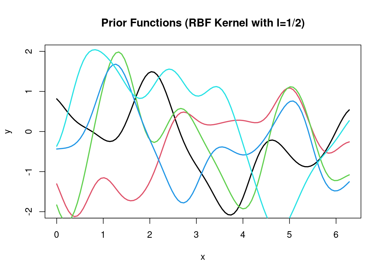
A widely used covariance function is \[ k(x, x^{\prime}) = \text{Cov}(x, x^{\prime}) = \sigma^2 e^{-\frac{ (x-x^{\prime})^2}{2 l^2}} \] This is known as the squared-exponential kernel or Radial-basis function (RBF) kernel.

Note that this kernel implies

• \(k(x, x) = \text{Var}(x) = \sigma^2\) and
• \(\text{Cor}(x, x^{\prime}) = e^{-\frac{ (x-x^{\prime})^2}{2 l^2}}\).

The parameter \(l\) in the RBF kernel is the length scale parameter and describes the “wigglyness” or “stiffness” of the resulting function. Small values of \(l\) correspond to more complex, more wiggly functions, and to low spatial correlation, as the correlation decreases quicker with distance, and large values correspond to more rigid, stiffer functions, with longer range spatial correlation (note that in a time series context this would be called autocorrelation).

There are many other kernel functions, including linear, polynomial or periodic kernels.

GP model

Nonlinear regression in the GP approach is conceptually very simple:

• start with multivariate prior
• then condition on the observed data
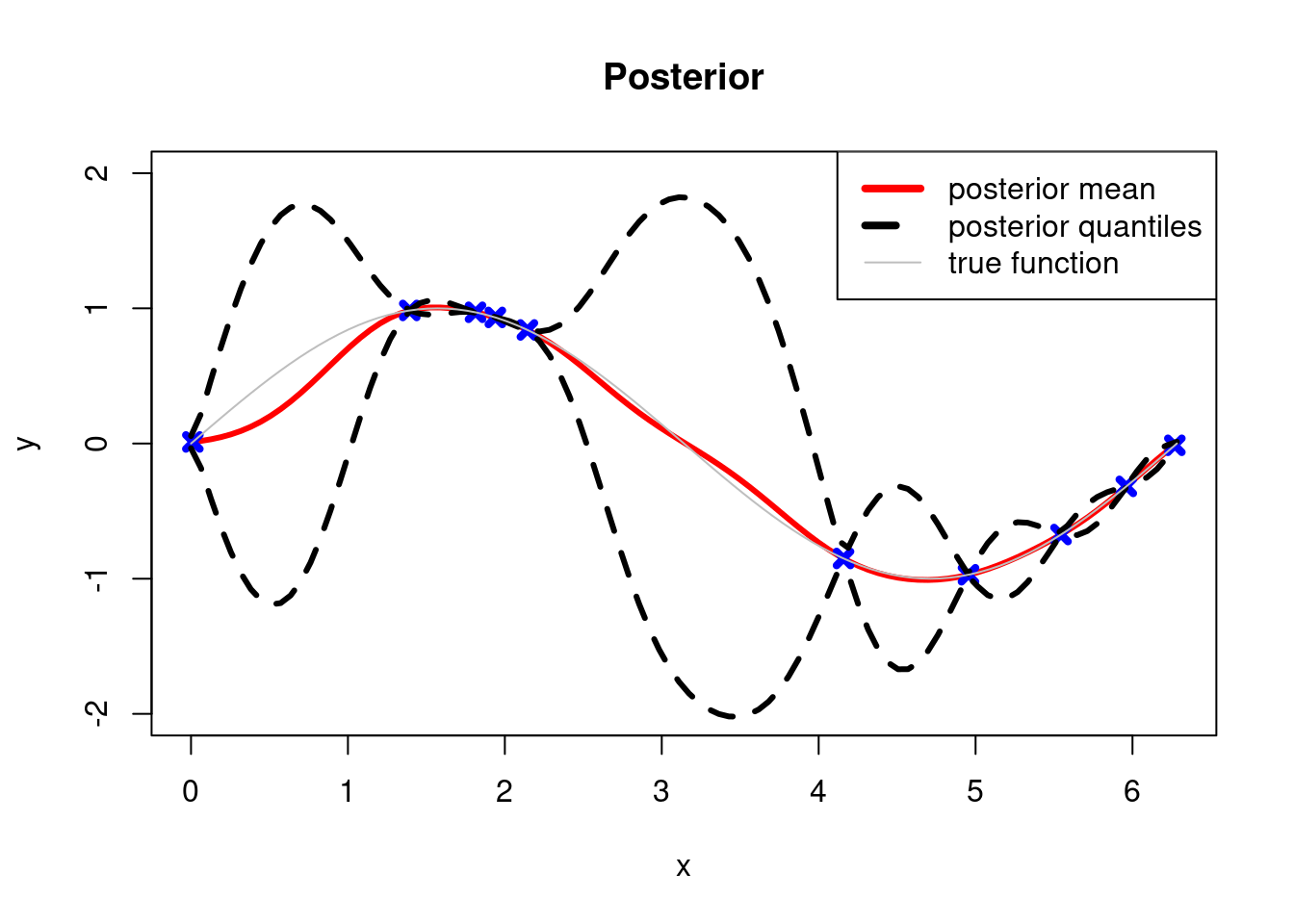
• the resulting conditional multivariate normal can used to predict the function values at any unobserved values
• the conditional variance can be used to compute credible intervals for predictions.

GP regression also provides a direct link with classical Bayesian linear regression (when using a linear kernel). Furthermore, GPs are also linked with neural networks as their limit in the case of an infinitely wide network (see section on neural networks).

Drawbacks of GPs: computationally expensive, typically \(O(n^3)\) because of the matrix inversion. However, there are now variations of GPs that help to overcome this issue (e.g. sparse GPs).

Gaussian process example

We now show how to apply Gaussian processes in R justing using standard matrix calculations.

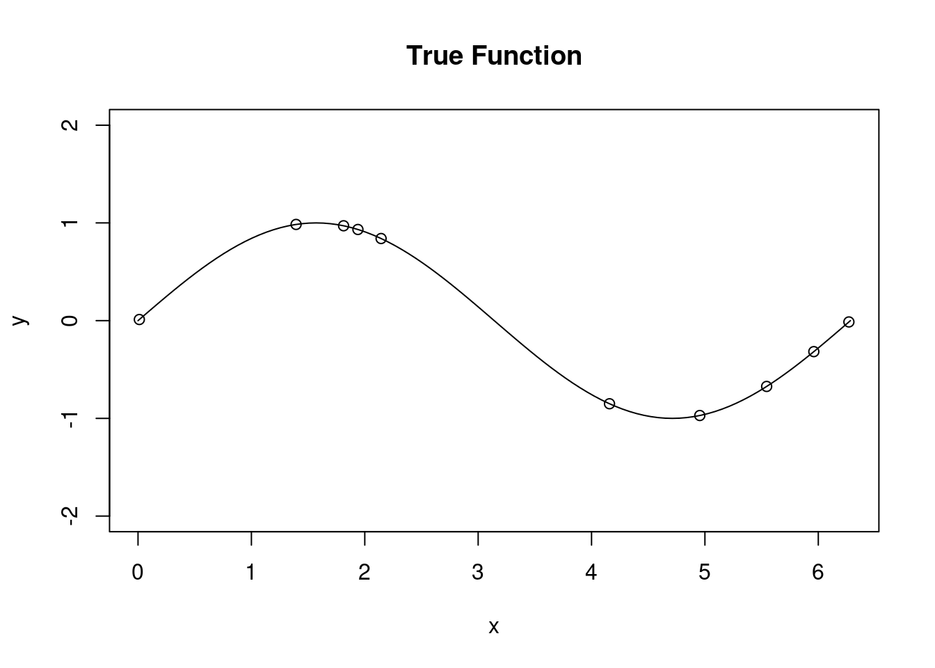
Our aim is to estimate the following nonlinear function from a number of observations. Note that initially we assume that there is no additional noise (so the observations lie directly on the curve): ::: {.cell}

truefunc = function(x) sin(x)
XLIM = c(0, 2*pi)
YLIM = c(-2, 2)

n2 = 10
x2 = runif(n2, min=XLIM[1], max=XLIM[2])
y2 = truefunc(x2)  # no noise

curve( truefunc(x), xlim=XLIM, ylim=YLIM, xlab="x", ylab="y", 
      main="True Function")
points(x2, y2)

::: Use the RFB kernel as the prior covariance and assume that the prior has mean zero: ::: {.cell}

# RBF kernel
rbfkernel = function(xa, xb, s2=1, l=1/2) s2*exp(-1/2*(xa-xb)^2/l^2)
kfun.mat = function(xavec, xbvec, FUN=rbfkernel) 
  outer(X=as.vector(xavec), Y=as.vector(xbvec), FUN=FUN)

# prior mean
mu.vec = function(x) rep(0, length(x))

::: Visualise the functions sampled from the multivariate normal prior: ::: {.cell}

# grid of x-values 
n1 = 100
x1 = seq(XLIM[1], XLIM[2], length.out=n1)

# unconditioned covariance and mean (unobserved samples x1)
K1 = kfun.mat(x1, x1)  
m1 = mu.vec(x1)

## sample functions from GP prior  
B = 5
library("MASS") # for mvrnorm
y1r = t(mvrnorm(B, mu = m1, Sigma=K1))
plot(x1, y1r[,1], type="l", lwd=2, ylab="y", xlab="x", ylim=YLIM, 
  main="Prior Functions (RBF Kernel with l=1/2)")
for(i in 2:B)
  lines(x1, y1r[,i], col=i, lwd=2)

:::

Compute the posterior mean and variance by conditioning on the observations: ::: {.cell}

# unconditioned covariance and mean (observed samples x2)
K2 = kfun.mat(x2, x2)
m2 = mu.vec(x2)
iK2 = solve(K2) # inverse

# cross-covariance
K12 = kfun.mat(x1, x2)

# Conditioning: x1 conditioned on x2
# conditional mean
m1.2 = m1 + K12 %*% iK2 %*% (y2 - m2)
# conditional variance
K1.2 = K1 - K12 %*% iK2 %*% t(K12)

:::

Plot the posterior mean and upper and lower bounds of a 95% credible interval:

# upper and lower CI
upper.bound = m1.2 + 1.96*sqrt(diag(K1.2))
lower.bound = m1.2 - 1.96*sqrt(diag(K1.2))

plot(x1, m1.2, type="l", xlim=XLIM, ylim=YLIM, col="red", lwd=3,
  ylab="y", xlab = "x", main = "Posterior")

points(x2,y2,pch=4,lwd=4,col="blue")
lines(x1,upper.bound,lty=2,lwd=3)
lines(x1,lower.bound,lty=2,lwd=3)
curve(truefunc(x), xlim=XLIM, add=TRUE, col="gray")

legend(x="topright", 
  legend=c("posterior mean", "posterior quantiles", "true function"),
  lty=c(1, 2, 1),lwd=c(4, 4, 1), col=c("red","black", "gray"), cex=1.0)

Finally, we can take into acount noise at the measured data points by adding an error term: ::: {.cell}

# add some noise
sdeps = 0.1
K2 = K2 + sdeps^2*diag(1,length(x2))

# update
iK2 = solve(K2) # inverse
m1.2 = m1 + K12 %*% iK2 %*% (y2 - m2)
K1.2 = K1 - K12 %*% iK2 %*% t(K12)
upper.bound = m1.2 + 1.96*sqrt(diag(K1.2))
lower.bound = m1.2 - 1.96*sqrt(diag(K1.2))

plot(x1, m1.2, type="l", xlim=XLIM, ylim=YLIM, col="red", lwd=3, 
  ylab="y", xlab = "x", main = "Posterior (with noise)")

points(x2,y2,pch=4,lwd=4,col="blue")
lines(x1,upper.bound,lty=2,lwd=3)
lines(x1,lower.bound,lty=2,lwd=3)
curve(truefunc(x), xlim=XLIM, add=TRUE, col="gray")

legend(x="topright", 
  legend=c("posterior mean", "posterior quantiles", "true function"),
  lty=c(1, 2, 1),lwd=c(4, 4, 1), col=c("red","black", "gray"), cex=1.0)

:::

Note that in the vicinity of data points the CIs are small and the further away from data the more uncertain the estimate of the underlying function becomes.

7.3 Neural networks

Another highly important class of models for nonlinear prediction (and nonlinear function approximation) are neural networks.

Relevant reading:

Please read: James et al. (2021) or James et al. (2023) Chapter 10 “Deep Learning”

History

Neural networks are actually relatively old models, going back to the 1950s.

Three phases of neural networks (NN)

• 1950/60: replicating functions of neurons in the brain (e.g. perceptron)
• 1980/90: neural networks as universal function approximators
• 2010—today: deep learning

The first phase was biologically inspired, the second phase focused on mathematical properties, and the current phase is pushed forward by advances in computer science and numerical optimisation:

• backpropagation algorithm
• efficient automatic symbolic differentiation (e.g. autograd)
• stochastic gradient descent algorithms (e.g. Adam)
• use of GPUs and TPUs (e.g. for linear algebra)
• availability of packages for symbolic tensor computations and deep learning.

Currently the most popular frameworks are:

• PyTorch (PyTorch Foundation, formerly Meta/Facebook)
• TensorFlow (Google Research)
• Flax / JAX (Google Research)

and high-level wrappers:

• skorch (scikit-learn wrapper for PyTorch)
• Keras 3 (for TensorFlow, JAX, and PyTorch)

Neural networks

Neural networks are essentially stacked systems of linear regressions, with nonlinear mappings between each layer, mapping the input to output via one or more layers of internal hidden nodes corresponding to internal latent variables:

• Each internal node is a nonlinear function of all or some of nodes in the previous layer
• Typically, the output of a node is computed using a non-linear activation function, such as the sigmoid function or a piecewise linear function (ReLU), from a linear combination of the input variables of that node.

A simple architecture is a feedforward network with a single hidden layer. More complex models are multilayer perceptrons and convolutional neural networks.

It can be shown that even simple network architectures can (with sufficient number of nodes) approximate any arbitrary non-linear function. This is called the universal function approximation property.

“Deep” neural networks have many layers, and the optimisation of their parameters requires advanced techniques (see above), with the objective function typically an empirical risk based on, e.g., squared error loss or cross-entropy loss. Neural networks are very highly parameterised models and therefore require lots of data for training, and typically also some form of regularisation (e.g. dropout).

As an extreme example, the neural network behind the ChatGPT 4 language model that is trained on essentially the whole freely accessible text available on the internet has an estimated 1.76 trillion (!) parameters (\(1.76 \times 10^{12}\)).

In the limit of an infinite width a single layer fully connected neural network becomes equivalent to a Gaussian process. This was first shown by R. M. Neal (1996)¹. More recently, this equivalence has also been demonstrated for other types of neural networks (with the kernel function of the GP being determined by the neural network architecture). This is formalised in the “neural tangent kernel” (NTK) framework.

Some of the statistical aspects of neural networks are not well understood. For example, there is the paradox that neural networks typically overfit the training data but still generalise well - this clearly violates the traditional understanding of bias-variance tradeoff for classical modelling in statistics and machine learning — see for example Belkin et al. (2019)². Some researchers argue that this contradiction can be resolved by better understanding the effective dimension of complex models. There is a lot of current research to explain this phenomenon of “multiple descent”, i.e. the decrease of prediction error for models with very many parameters. A further topic is robustness of the predictions, which is also caused by overfitting. It is well known that neural networks can sometimes be “fooled” by so-called adversarial examples, e.g., the classification of a sample may change if a small amount of noise is added to the test data.

Learning more about deep learning

A good place to learn more about the concepts of deep learning is the book “Understanding Deep Learning” by Prince (2023) available online at https://udlbook.github.io/udlbook/. For actual application in computer code using various software frameworks the book “Dive Into Deep Learning” by Zhang et al. (2023) available online at https://d2l.ai is recommended.

James, G., D. Witten, T. Hastie, and R. Tibshirani. 2021. An Introduction to Statistical Learning with Applications in R. 2nd ed. Springer. https://doi.org/10.1007/978-1-0716-1418-1.

James, G., D. Witten, T. Hastie, R. Tibshirani, and J. Taylor. 2023. An Introduction to Statistical Learning with Applications in Python. Springer. https://doi.org/10.1007/978-3-031-38747-0.

Prince, S. J. D. 2023. Understanding Deep Learning. MIT Press. https://mitpress.mit.edu/9780262048644/understanding-deep-learning/.

Rogers, S., and M. Girolami. 2017. A First Course in Machine Learning. 2nd ed. Chapman; Hall / CRC. https://doi.org/10.1201/9781315382159.

Zhang, A., Z. C. Lipton, M. Li, and A. J. Smola. 2023. Dive into Deep Learning. https://d2l.ai.

---

1. Neal, R. M. 1996. Bayesian Learning for Neural Networks. Springer. https://doi.org/10.1007/978-1-4612-0745-0

2. Belkin, M. et al. 2019. Reconciling modern machine-learning practice and the classical bias–variance trade-off. PNAS 116: 15849–15854. https://doi.org/10.1073/pnas.1903070116