2 Multivariate estimation
2.1 Overview
In practical application of multivariate normal model we need to learn its parameters from observed data points:
\[\boldsymbol x_1,\boldsymbol x_2,...,\boldsymbol x_n \stackrel{\text{iid}}\sim F_{\boldsymbol \theta}\]
We first consider the case when there are many measurements available (\(n\) large), and then subsequently the case when the number of data points \(n\) is small compared to the dimensions and the number of parameters.
In a previous course in year 2 (see MATH27720 Statistics 2) the method of maximum likelihood as well as the essentials of Bayesian statistics were introduced. Below we apply these approaches to the problem of estimating the parameters of the multivariate normal distribution and also show how the main Bayesian modelling strategies extend to the multivariate case.
2.2 Empirical estimates
General principle
For large \(n\) we have thanks to the law of large numbers: \[\underbrace{F}_{\text{true}} \approx \underbrace{\widehat{F}_n}_{\text{empirical}}\]
We now would like to estimate \(A\) which is a functional \(A=m(F)\) of the distribution \(F\) — recall that a functional is a function that takes another function as argument. For example all standard distributional summaries such as the mean, the median etc. are derived from \(F\) and hence are functionals of \(F\).
The empirical estimate is obtained by replacing the unknown true distribution \(F\) with the observed empirical distribution: \(\hat{A} = m(\widehat{F}_n)\).
For example, the expectation of a random variable is approximated/estimated as the average over the observations: \[\text{E}_F(\boldsymbol x) \approx \text{E}_{\widehat{F}_n}(\boldsymbol x) = \frac{1}{n}\sum^{n}_{k=1} \boldsymbol x_k\] \[\text{E}_F(g(\boldsymbol x)) \approx \text{E}_{\widehat{F}_n}(g(\boldsymbol x)) = \frac{1}{n}\sum^{n}_{k=1} g(\boldsymbol x_k)\]
Simple recipe to obtain an empirical estimator: simply replace the expectation operator by the sample average.
What does this work: the empirical distribution \(\widehat{F}_n\) is the nonparametric maximum likelihood estimate of \(F\) (see below for likelihood estimation).
Note: the approximation of \(F\) by \(\widehat{F}_n\) is also the basis other approaches such as Efron’s bootstrap method (1979) 1.
Empirical estimates of mean and covariance
Recall the definitions: \[ \boldsymbol \mu= \text{E}(\boldsymbol x) \] and \[ \boldsymbol \Sigma= \text{E}\left( (\boldsymbol x-\boldsymbol \mu) (\boldsymbol x-\boldsymbol \mu)^T \right) \]
For the empirical estimate we replace the expectations by the corresponding sample averages.
These resulting estimators can be written in three different ways:
Vector notation:
\[\hat{\boldsymbol \mu} = \frac{1}{n}\sum^{n}_{k=1} \boldsymbol x_k\]
\[ \widehat{\boldsymbol \Sigma} = \frac{1}{n}\sum^{n}_{k=1} (\boldsymbol x_k-\hat{\boldsymbol \mu}) (\boldsymbol x_k-\hat{\boldsymbol \mu})^T = \frac{1}{n}\sum^{n}_{k=1} \boldsymbol x_k \boldsymbol x_k^T - \hat{\boldsymbol \mu} \hat{\boldsymbol \mu}^T \]
Component notation:
The corresponding component notation with \(\boldsymbol X= (x_{ki})\) and following the statistics convention with samples contained in rows of \(\boldsymbol X\) we get:
\[\hat{\mu}_i = \frac{1}{n}\sum^{n}_{k=1} x_{ki}\]
\[\hat{\sigma}_{ij} = \frac{1}{n}\sum^{n}_{k=1} (x_{ki}-\hat{\mu}_i) ( x_{kj}-\hat{\mu}_j )\]
\[\hat{\boldsymbol \mu}=\begin{pmatrix} \hat{\mu}_{1} \\ \vdots \\ \hat{\mu}_{d} \end{pmatrix}, \widehat{\boldsymbol \Sigma} = (\hat{\sigma}_{ij})\]
Variance estimate:
\[\hat{\sigma}_{ii} = \frac{1}{n}\sum^{n}_{k=1} \left(x_{ki}-\hat{\mu}_i\right)^2\] Note the factor \(\frac{1}{n}\) (not \(\frac{1}{n-1}\))
Data matrix notation:
The empirical mean and covariance can also be written in terms of the data matrix \(\boldsymbol X\).
If the data matrix \(\boldsymbol X\) follows the statistics convention we can write
\[\hat{\boldsymbol \mu} = \frac{1}{n} \boldsymbol X^T \mathbf 1_n\]
\[\widehat{\boldsymbol \Sigma} = \frac{1}{n} \boldsymbol X^T \boldsymbol X- \hat{\boldsymbol \mu} \hat{\boldsymbol \mu}^T\]
On the other hand, if \(\boldsymbol X\) follows the engineering convention with samples in columns the estimators are written as:
\[\hat{\boldsymbol \mu} = \frac{1}{n} \boldsymbol X\mathbf 1_n\]
\[\widehat{\boldsymbol \Sigma} = \frac{1}{n} \boldsymbol X\boldsymbol X^T - \hat{\boldsymbol \mu} \hat{\boldsymbol \mu}^T\]
To avoid confusion when using matrix or component notation you need to always state which convention is used! In these notes we exlusively follow the statistics convention.
2.3 Maximum likelihood estimation
General principle
R.A. Fisher (1922) 2: model-based estimators using the density or probability mass function
Log-likelihood function:
Observing data \(D=\{ \boldsymbol x_1, \ldots, \boldsymbol x_n\}\) the log-likelihood function is
\[\log L(\boldsymbol \theta| D ) = \sum^{n}_{k=1} \underbrace{\log f}_{\text{log-density}}(\boldsymbol x_k |\boldsymbol \theta)\]
Maximum likelihood estimate: \[\hat{\boldsymbol \theta}_{\text{ML}}=\underset{\boldsymbol \theta}{\arg\,\max} \log L(\boldsymbol \theta| D)\]
Maximum likelihood (ML) finds the parameters that make the observed data most likely (it does not find the most probable model!)
Recall from MATH27720 Statistics 2 that maximum likelihood is closely linked to minimising the Kullback-Leibler (KL) divergence \(D_{\text{KL}}(F, F_{\boldsymbol \theta})\) between the unknown true model \(F\) and the specified model \(F_{\boldsymbol \theta}\). Specifically, for large sample size \(n\) the model \(F_{\hat{\boldsymbol \theta}}\) fit by maximum likelihood is indeed the model that is closest to \(F\).
Correspondingly, the great appeal of maximum likelihood estimates (MLEs) is that they are optimal for large \(\mathbf{n}\), i.e. so that for large sample size no estimator can be constructed that outperforms the MLE (note the emphasis on “for large \(n\)”!). A further advantage of the method of maximum likelihood is that it does not only provide a point estimate but also the asymptotic error (via the observed Fisher information which is related to the curvature of the log-likelihood function).
Maximum likelihood estimates of the parameters of the multivariate normal distribution
We now derive the MLE of the parameters \(\boldsymbol \mu\) and \(\boldsymbol \Sigma\) of the multivariate normal distribution. The corresponding log-likelihood function is \[ \begin{split} \log L(\boldsymbol \mu, \boldsymbol \Sigma| D) & = \sum_{k=1}^n \log f( \boldsymbol x_k | \boldsymbol \mu, \boldsymbol \Sigma) \\ & = -\frac{n d}{2} \log(2\pi) -\frac{n}{2} \log \det(\boldsymbol \Sigma) - \frac{1}{2} \sum_{k=1}^n (\boldsymbol x_k-\boldsymbol \mu)^T \boldsymbol \Sigma^{-1} (\boldsymbol x_k-\boldsymbol \mu) \,.\\ \end{split} \] Written in terms of the precision matrix \(\boldsymbol \Omega= \boldsymbol \Sigma^{-1}\) this becomes \[ \log L(\boldsymbol \mu, \boldsymbol \Omega| D) = -\frac{n d}{2} \log(2\pi) +\frac{n}{2} \log \det(\boldsymbol \Omega) - \frac{1}{2} \sum_{k=1}^n (\boldsymbol x_k-\boldsymbol \mu)^T \boldsymbol \Omega(\boldsymbol x_k-\boldsymbol \mu) \,. \] First, to find the MLE for \(\boldsymbol \mu\) we compute the derivative with regard to the vector \(\boldsymbol \mu\) \[ \frac{\partial \log L(\boldsymbol \mu, \boldsymbol \Omega| D) }{\partial \boldsymbol \mu}= \sum_{k=1}^n (\boldsymbol x_k-\boldsymbol \mu)^T \boldsymbol \Omega\] noting that \(\boldsymbol \Omega\) is symmetric. Setting this equal to zero we get \(\sum_{k=1}^n \boldsymbol x_k = n \hat{\boldsymbol \mu}_{ML}\) and thus \[\hat{\boldsymbol \mu}_{ML} = \frac{1}{n} \sum_{k=1}^n \boldsymbol x_k\,.\]
Next, to obtain the MLE for \(\boldsymbol \Omega\) we compute the derivative with regard to the matrix \(\boldsymbol \Omega\) \[\frac{\partial \log L(\boldsymbol \mu, \boldsymbol \Omega| D) }{\partial \boldsymbol \Omega}=\frac{n}{2}\boldsymbol \Omega^{-1} - \frac{1}{2} \sum_{k=1}^n (\boldsymbol x_k-\boldsymbol \mu) (\boldsymbol x_k-\boldsymbol \mu)^T\]. Setting this equal to zero and substituting the MLE for \(\boldsymbol \mu\) we get \[\widehat{\boldsymbol \Omega}^{-1}_{ML}= \frac{1}{n} \sum_{k=1}^n (\boldsymbol x_k-\hat{\boldsymbol \mu}) (\boldsymbol x_k-\hat{\boldsymbol \mu})^T=\widehat{\boldsymbol \Sigma}_{ML}\,.\]
See the supplementary Matrix Refresher notes for the relevant formulas in vector and matrix calculus.
Therefore, the MLEs are identical to the empirical estimates.
Note the factor \(\frac{1}{n}\) in the MLE of the covariance matrix.
2.4 Sampling distribution of the empirical / maximum likelihood estimates
With \(\boldsymbol x_1,...,\boldsymbol x_n \sim N_d(\boldsymbol \mu, \boldsymbol \Sigma)\) one can find the exact distributions of the estimators. The sample average is denoted by \(\bar{\boldsymbol x}= \frac{1}{n}\sum_{i=1}^n \boldsymbol x_i\)
1. Distribution of the estimate of the mean:
The empirical estimate of the mean is normally distributed:
\[\hat{\boldsymbol \mu}_{ML}=\bar{\boldsymbol x} \sim N_d\left(\boldsymbol \mu, \frac{\boldsymbol \Sigma}{n}\right)\] Since \(\text{E}(\hat{\boldsymbol \mu}_{ML}) = \boldsymbol \mu\Longrightarrow \hat{\boldsymbol \mu}_{ML}\) is unbiased.
2. Distribution of the covariance estimate:
The empirical and unbiased estimate of the covariance matrix is Wishart distributed:
Case of unknown mean \(\boldsymbol \mu\) (estimated by \(\bar{\boldsymbol x}\)):
\[\widehat{\boldsymbol \Sigma}_{ML} = \frac{1}{n}\sum_{i=1}^n (\boldsymbol x_i -\bar{\boldsymbol x})(\boldsymbol x_i -\bar{\boldsymbol x})^T \sim \text{Wis}\left(\frac{\boldsymbol \Sigma}{n}, n-1\right)\]
Since \(\text{E}(\widehat{\boldsymbol \Sigma}_{ML}) = \frac{n-1}{n}\boldsymbol \Sigma\) \(\Longrightarrow \widehat{\boldsymbol \Sigma}_{ML}\) is biased, with \(\text{Bias}(\widehat{\boldsymbol \Sigma}_{ML} ) = \boldsymbol \Sigma- \text{E}(\widehat{\boldsymbol \Sigma}_{ML}) = -\frac{\boldsymbol \Sigma}{n}\).
Easy to make unbiased: \(\widehat{\boldsymbol \Sigma}_{UB} = \frac{n}{n-1}\widehat{\boldsymbol \Sigma}_{ML}= \frac{1}{n-1}\sum^n_{k=1}\left(\boldsymbol x_k-\bar{\boldsymbol x}\right)\left(\boldsymbol x_k-\bar{\boldsymbol x}\right)^T\) which is distributed as \[\widehat{\boldsymbol \Sigma}_{UB} \sim \text{Wis}\left(\frac{\boldsymbol \Sigma}{n-1}, n-1\right)\]
Hence \(\text{E}(\widehat{\boldsymbol \Sigma}_{UB}) = \boldsymbol \Sigma\) \(\Longrightarrow \widehat{\boldsymbol \Sigma}_{UB}\) is unbiased.
But unbiasedness of an estimator is not a very relevant criterion in multivariate statistics, especially when the number of samples is small compared to the dimension (see further below).
Covariance estimator for known mean \(\boldsymbol \mu\):
\[\frac{1}{n}\sum_{i=1}^n (\boldsymbol x_i -\boldsymbol \mu)(\boldsymbol x_i -\boldsymbol \mu)^T \sim \text{Wis}\left(\frac{\boldsymbol \Sigma}{n}, n\right)\]
2.5 Small sample estimation
Problems with maximum likelihood in small sample settings and high dimensions
Modern data is high dimensional!
Data sets with \(n<d\), i.e. high dimension \(d\) and small sample size \(n\) are now common in many fields, e.g., medicine, biology but also finance and business analytics.
\[n = 100 \, \text{(e.g., patients/samples)}\] \[d = 20000 \, \text{(e.g., genes/SNPs/proteins/variables)}\] Reasons:
- the number of measured variables is increasing quickly with technological advances (e.g. genomics)
- but the number of samples cannot be similary increased (for cost and ethical reasons)
General problems of MLEs:
- ML estimators are optimal only if sample size is large compared to the number of parameters. However, this optimality is not any more valid if sample size is moderate or smaller than the number of parameters.
- If there is not enough data the ML estimate overfits. This means ML fits the current data perfectly but the resulting model does not generalise well (i.e. model will perform poorly in prediction)
- If there is a choice between different models with different complexity ML will always select the model with the largest number of parameters.
-> for high-dimensional data with small sample size maximum likelihood estimation does not work!!!
History of Statistics:
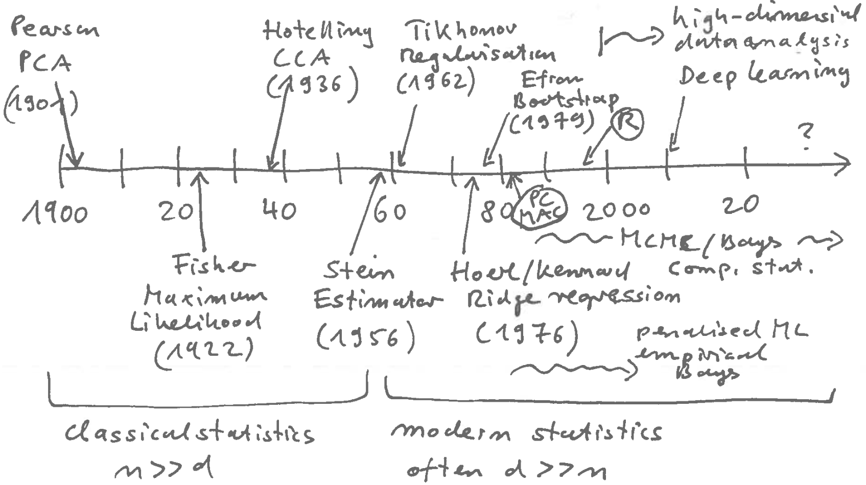
Much of modern statistics (from 1960 onwards) is devoted to the development of inference and estimation techniques that work with complex, high-dimensional data (cf. Figure 2.1).
- Maximum likelihood is a method from classical statistics (time up to about 1960).
- From 1960 modern (computational) statistics emerges, starting with “Stein Paradox” (1956): Charles Stein showed that in a multivariate setting ML estimators are dominated by (= are always worse than) shrinkage estimators!
- For example, there is a shrinkage estimator for the mean that is better (in terms of MSE) than the average (which is the MLE)!
Modern statistics has developed many different (but related) methods for use in high-dimensional, small sample settings:
- regularised estimators
- shrinkage estimators
- penalised maximum likelihood estimators
- Bayesian estimators
- Empirical Bayes estimators
- KL / entropy-based estimators
Most of this is out of scope for our class, but will be covered in advanced statistical courses.
Next, we describe a simple regularised estimator for the estimation of the covariance that we will use later (i.e. in classification).
Estimation of covariance matrix in small sample settings
Problems with ML estimate of \(\boldsymbol \Sigma\)
\(\Sigma\) has O(\(d^2\)) number of parameters! \(\Longrightarrow \hat{\boldsymbol \Sigma}^{\text{MLE}}\) requires a lot of data! \(n\gg d \text{ or } d^2\)
if \(n < d\) then \(\hat{\boldsymbol \Sigma}\) is positive semi-definite (even if the true \(\Sigma\) is positive definite!)
\(\Longrightarrow \hat{\boldsymbol \Sigma}\) will have vanishing eigenvalues (some \(\lambda_i=0\)) and thus cannot be inverted and is singular!
Note that in many expression in multivariate statistics we actually need to use the inverse of the covariance matrix, e.g., in the density of the multivariate normal distribution, so it is essential that we obtain a non-singular invertible estimate of the covariance matrix.
Making the ML estimate of \(\boldsymbol \Sigma\) invertible
There is a simple numerical trick credited to A. N. Tikhonov to make \(\hat{\boldsymbol \Sigma}\) invertible, by adding a small number (say \(\varepsilon=10^{-6}\) to the diagonal elements of \(\hat{\boldsymbol \Sigma}\): \[ \boldsymbol S_{\text{Tik}} = \hat{\boldsymbol \Sigma} + \varepsilon \boldsymbol I \]
The resulting \(\boldsymbol S_{\text{Tik}}\) is positive definite because the sum of a symmetric positive definite matrix (\(\varepsilon \boldsymbol I\)) and a symmetric positive semi-definite matrix (\(\hat{\boldsymbol \Sigma}\)) is always positive definite.
However, while this simple regularisation results in an invertible matrix the estimator itself has not improved over the MLE, and the matrix \(\boldsymbol S_{\text{Tik}}\) will also be poorly conditioned (i.e. large condition number).
Simple regularised estimate of \(\boldsymbol \Sigma\)
Regularised estimator \(\boldsymbol S^\ast\) = convex combination of \(\boldsymbol S= \hat{\boldsymbol \Sigma}^\text{MLE}\) and \(\boldsymbol I_d\) (identity matrix) to get
Regularisation: \[ \underbrace{\boldsymbol S^\ast}_{\text{regularised estimate}} = (1-\lambda)\underbrace{\boldsymbol S}_{\text{ML estimate}} +\underbrace{\lambda}_{\text{shrinkage intensity}} \, \underbrace{\boldsymbol I_d}_{\text{target}}\]
Idea: choose \(\lambda \in [0,1]\) such that \(\boldsymbol S^\ast\) is better (e.g. in terms of MSE) than both \(\boldsymbol S\) and \(\boldsymbol I_d\). Note that \(\lambda\) does not need to be small like \(\varepsilon\).
This form of estimator is corresponds to computing the mean of the Bayesian posterior by directly shrinking the MLE towards a prior mean (target): \[ \underbrace{\boldsymbol S^\ast}_{\text{posterior mean}} = \underbrace{\lambda \boldsymbol I_d}_{\text{prior information}} + (1-\lambda)\underbrace{\boldsymbol S}_{\text{data summarised by maximum likelihood}} \]
- Prior information helps to infer \(\boldsymbol \Sigma\) even in small samples.
- also called shrinkage estimator since the off-diagonal entries are shrunk towards zero.
- this type of linear shrinkage/regularisation is natural for exponential family models (Diaconis and Ylvisaker, 1979).
- Instead of a diagonal target other options are possible, e.g. block-diagonal or banded covariances.
- If \(\lambda\) is not prespecified but learned from data (see below) then the resulting estimate is an empirical Bayes estimator.
- The resulting estimate will typically be biased as mixing in the target will increase the bias.
How to find optimal shrinkage / regularisation parameter \(\lambda\)?

One way to do this is to chose \(\lambda\) to minimise \(\text{MSE}\) (Mean Squared Error) — see Figure 2.2. This is also called L2 regularisation or Ridge regularisation.
Bias-variance trade-off: \(\text{MSE}\) is composed of squared bias and variance.
\[\text{MSE}(\theta) = \text{E}((\hat{\theta}-\theta)^2) = \text{Bias}(\hat{\theta})^2 + \text{Var}(\hat{\theta})\] with \(\text{Bias}(\hat{\theta}) = \text{E}(\hat{\theta})-\theta\)
\(\boldsymbol S\): ML estimate, many parameters, low bias, high variance
\(\boldsymbol I_d\): “target”, no parameters, high bias, low variance
\(\Longrightarrow\) reduce high variance of \(\boldsymbol S\) by introducing a bit of bias through \(\boldsymbol I_d\)!
\(\Longrightarrow\) overall, \(\text{MSE}\) is decreased
Challenge: since we don’t know the true \(\boldsymbol \Sigma\) we cannot actually compute the \(\text{MSE}\) directly but have to estimate it! How is this done in practise?
- by cross-validation (=resampling procedure)
- by using some analytic approximation (e.g. Stein’s formula)
In Worksheet 3 the empirical estimator of covariance is compared with the regularised covariance estimator implemented in the R package “corpcor”. This uses a regularisation similar as above (but for the correlation rather than the covariance matrix) and it employs an analytic data-adaptive estimate of the shrinkage intensity \(\lambda\). This estimator is a variant of an empirical Bayes / James-Stein estimator (see MATH27720 Statistics 2).
2.6 Full Bayesian multivariate modelling
See also the section about multivariate distributions in the Probability and Distribution refresher for details about the distributions used below.
Three main scenarios
As discussed in MATH27720 Statistics 2 there are three main Bayesian models in the univariate case that cover a large range of applications:
- the beta-binomial model to estimate proportions
- the normal-normal model to estimate means
- the inverse gamma-normal model to estimate variances
Below we briefly sketch the extensions of these three elementary models to the multivariate case.
Dirichlet-multinomial model
This generalises the univariate beta-binomial model.
The Dirichlet distribution \(\text{Dir}(\boldsymbol \alpha)\) is useful as conjugate prior and posterior distribution for the parameters of a categorical distribution.
Data: \(D=\{\boldsymbol x_1, \ldots, \boldsymbol x_n\}\) with \(\boldsymbol x_i \sim \text{Cat}(\boldsymbol \pi)\)
MLE: \(\hat{\boldsymbol \pi}_{ML} = \frac{1}{n} \sum_{i=1}^n \boldsymbol x_i\)
Prior parameters (Dirichlet in mean parametrisation): concentration parameter \(k_0\), mean parameter \(\boldsymbol \pi_0\),
\[\boldsymbol \pi\sim \text{Dir}(\boldsymbol \pi_0 k_0)\] \[\text{E}(\boldsymbol \pi) = \boldsymbol \pi_0\]Posterior parameters: \(k_1 = k_0+n\), \(\boldsymbol \pi_1 = \lambda \boldsymbol \pi_0 + (1-\lambda) \, \hat{\boldsymbol \pi}_{ML}\) with \(\lambda = \frac{k_0}{k_1}\)
\[\boldsymbol \pi\,| \, D \sim \text{Dir}(\boldsymbol \pi_1 k_1)\] \[\text{E}(\boldsymbol \pi\,| \, D) = \boldsymbol \pi_1\]Equivalent update rule (for Dirichlet \(\boldsymbol \alpha\) parameter): \(\boldsymbol \alpha_0\) \(\rightarrow\) \(\boldsymbol \alpha_1 = \boldsymbol \alpha_0 + \sum_{i=1}^n \boldsymbol x_i = \boldsymbol \alpha_0 + n \hat{\boldsymbol \pi}_{ML}\)
Multivariate normal-normal model
This generalises the univariate normal-normal model.
The multivariate normal distribution \(N_d(\boldsymbol \mu, \boldsymbol \Sigma)\) is useful as conjugate prior and posterior distribution of the mean:
Data: \(D =\{\boldsymbol x_1, \ldots, \boldsymbol x_n\}\) with \(\boldsymbol x_i \sim N_d(\boldsymbol \mu, \boldsymbol \Sigma)\) with known mean \(\boldsymbol \Sigma\)
MLE: \(\widehat{\boldsymbol \mu}_{ML} = \frac{1}{n} \sum_{i=1}^n \boldsymbol x_i\)
Prior parameters: \(k_0\), \(\boldsymbol \mu_0\) \[\boldsymbol \mu\sim N_d\left(\boldsymbol \mu_0, \frac{\boldsymbol \Sigma}{k_0}\right)\] \[\text{E}(\boldsymbol \mu) = \boldsymbol \mu_0\]
Posterior parameters: \(k_1 = k_0+n\), \(\boldsymbol \mu_1 = \lambda \boldsymbol \mu_0 + (1-\lambda) \widehat{\boldsymbol \mu}_{ML}\) with \(\lambda = \frac{k_0}{k_1}\)
\[\boldsymbol \mu\, |\, D \sim N_d\left( \boldsymbol \mu_1, \frac{\boldsymbol \Sigma}{k_1} \right)\] \[\text{E}(\boldsymbol \mu\, |\, D) = \boldsymbol \mu_1\]
Inverse Wishart-normal model
This generalises the univariate inverse gamma-normal model for the variance.
The inverse Wishart distribution \(\text{IW}\left(\boldsymbol \Psi, k\right)\) is useful as conjugate prior and posterior distribution of the covariance:
Data: \(D =\{\boldsymbol x_1, \ldots, \boldsymbol x_n\}\) with \(\boldsymbol x_i \sim N_d(\boldsymbol \mu, \boldsymbol \Sigma)\) with known mean \(\boldsymbol \mu\)
MLE: \(\widehat{\boldsymbol \Sigma}_{ML} = \frac{1}{n} \sum_{i=1}^n (\boldsymbol x_i-\boldsymbol \mu)(\boldsymbol x_i-\boldsymbol \mu)^T\)
Prior parameters: \(\kappa_0\), \(\boldsymbol \Sigma_0\) \[\boldsymbol \Sigma\sim \text{IW}\left( \kappa_0 \boldsymbol \Sigma_0 \, , \, \kappa_0+d+1\right)\] \[\text{E}(\boldsymbol \Sigma) = \boldsymbol \Sigma_0\]
Posterior parameters: \(\kappa_1 = \kappa_0+n\), \(\boldsymbol \Sigma_1 = \lambda \boldsymbol \Sigma_0 + (1-\lambda) \widehat{\boldsymbol \Sigma}_{ML}\) with \(\lambda = \frac{\kappa_0}{\kappa_1}\)
\[\boldsymbol \Sigma\, |\, D \sim \text{IW}\left( \kappa_1 \boldsymbol \Sigma_1 \, , \, \kappa_1+d+1\right)\] \[\text{E}(\boldsymbol \Sigma\, |\, D) = \boldsymbol \Sigma_1\]Equivalent update rule using \(\boldsymbol \Psi\) and \(k\) as parameters: \(k_0\) \(\rightarrow\) \(k_1 = k_0+n\), \(\boldsymbol \Psi_0\) \(\rightarrow\) \(\boldsymbol \Psi_1 = \boldsymbol \Psi_0 + \sum_{i=1}^n (\boldsymbol x_i-\boldsymbol \mu)(\boldsymbol x_i-\boldsymbol \mu)^T = \boldsymbol \Psi_0 + n \widehat{\boldsymbol \Sigma}_{ML}\)
2.7 Conclusion
- Multivariate models are often high-dimensional with large number of parameters but often only a small number of samples are available. In this instance it is useful (and often necessary) to introduce additional information (via priors or by regularisation).
- Unbiased estimation, a highly valued property in classical univariate statistics when sample size is large and number of parameters is small, is typically not a good idea in multivariate settings and often leads to poor estimators.
- Regularisation introduces bias and reduces variance, minimising overall MSE. Likewise, Bayesian estimators also introduce bias and regularise (via the prior) and thus are useful in multivariate settings.
Efron, B. 1979. Bootstrap methods: Another look at the jackknife. The Annals of Statistics 7:1–26. https://doi.org/10.1214/aos/1176344552↩︎
Fisher, R. A. 1922. On the mathematical foundations of theoretical statistics. Philosophical Transactions of the Royal Society A 222:309–368. https://doi.org/10.1098/rsta.1922.0009↩︎