2 Probability
2.1 Random variables
A random variable describes a random experiment. The set of all possible outcomes is the sample space of the random variable and is denoted by \(\Omega\). If \(\Omega\) is countable then the random variable is discrete, otherwise it is continuous. For a discrete random variable the sample space \(\Omega = \{\omega_1, \omega_2, \ldots\}\) is composed of a finite or infinite number of elementary outcomes \(\omega_i\).
An event \(A \subseteq \Omega\) is a subset of \(\Omega\). This includes as special cases the complete set \(\Omega\) (“certain event”) and the empty set \(\emptyset\) (“impossible event”). The set of all possible events is denoted by \(\mathcal{F}\). The complementary event \(A^C = \Omega \setminus A\) is the complement of the set \(A\) in the sample space \(\Omega\). Two events \(A_1\) and \(A_2\) are mutually exclusive if the sets are disjoint with \(A_1 \cap A_2 = \emptyset\).
For a discrete random variable, the elementary outcomes \(\omega_i\) are referred to as elementary events, and they are all mutually exclusive. An event \(A\) consists of a number of elementary events \(\omega_i \in A\) and the complementary event is given by \(A^C = \{\omega_i \in \Omega: \omega_i \notin A\}\).
The probability of an event \(A\) is denoted by \(\operatorname{Pr}(A)\). Broadly, \(\operatorname{Pr}(A)\) provides a measure of the size of the set \(A\) relative to the set \(\Omega\). The probability measure \(\operatorname{Pr}(A)\) satisfies the three axioms of probability:
- \(\operatorname{Pr}(A) \geq 0\), probabilities are nonnegative,
- \(\operatorname{Pr}(\Omega) = 1\), the certain event has probability 1, and
- \(\operatorname{Pr}(A_1 \cup A_2 \cup \ldots) = \sum_i \operatorname{Pr}(A_i)\), the probability of countable mutually exclusive events \(A_i\) is additive.
This implies
- \(\operatorname{Pr}(A) \leq 1\), probability values lie within the range \([0,1]\),
- \(\operatorname{Pr}(A^C) = 1 - \operatorname{Pr}(A)\), the probability of the complement, and
- \(\operatorname{Pr}(\emptyset) = 0\), the impossible event has probability 0.
From the above it is evident that probability is closely linked to set theory, in particular to measure theory which serves as the theoretical foundations of probability and generalisations. For instance, if \(\operatorname{Pr}(\emptyset) = 0\) is assumed instead of \(\operatorname{Pr}(\Omega) = 1\), this leads to the axioms for a positive measure (of which probability is a special case).
2.2 Conditional probability
Consider two events \(A\) and \(B\), which may not be be mutually exclusive. The probability of the event “\(A\) and \(B\)” is given by the probability of the set intersection \(\operatorname{Pr}(A \cap B)\). The probability of the event “\(A\) or \(B\)” is given by the probability of the set union \[ \operatorname{Pr}(A \cup B) = \operatorname{Pr}(A) + \operatorname{Pr}(B) - \operatorname{Pr}(A \cap B)\,. \] This identity follows from the axioms.
The conditional probability of event \(A\) assuming event \(B\) has occurred is given by \[ \operatorname{Pr}(A | B) = {\operatorname{Pr}( A \cap B) \over \operatorname{Pr}(B)} \] Essentially, now \(B\) acts as the new sample space relative to which \(A\) is measured, restricting it from \(\Omega\). Note that \(\operatorname{Pr}(A | B)\) is generally not the same as \(\operatorname{Pr}(B | A)\), see Bayes’ theorem below.
Importantly, it can be seen that any probability may be viewed as conditional, namely relative to \(\Omega\) as \(\operatorname{Pr}(A) = \operatorname{Pr}(A| \Omega)\).
From the definition of conditional probability we derive the product rule \[ \begin{split} \operatorname{Pr}( A \cap B) &= \operatorname{Pr}(A | B)\, \operatorname{Pr}(B) \\ &= \operatorname{Pr}(B | A)\, \operatorname{Pr}(A) \end{split} \] which in turn yields Bayes’ theorem \[ \operatorname{Pr}(A | B ) = \operatorname{Pr}(B | A) { \operatorname{Pr}(A) \over \operatorname{Pr}(B)} \] This theorem is useful for changing the order of conditioning and it plays a key role in Bayesian statistics.
If \(\operatorname{Pr}( A \cap B) = \operatorname{Pr}(A) \, \operatorname{Pr}(B)\) then the two events \(A\) and \(B\) are independent with \(\operatorname{Pr}(A | B ) = \operatorname{Pr}(A)\) and \(\operatorname{Pr}(B | A ) = \operatorname{Pr}(B)\).
2.3 Probability mass and density function
The distribution (or law) of a random variable \(x\) with sample space \(\Omega\) is the probability measure that assigns probabilities to values or ranges of \(x\). This is done in practise by employing probability mass functions (pmf, for discrete random variables) or probability density functions (pdf, for continuous random variables).
The scalar random variable \(x\) is written in lowercase plain font. We use the same symbol \(x\) for both the random variable and its realisations.1
For a discrete random variable we define the event \(A = \{x: x=a\} = \{a\}\) (corresponding to a single elementary event) and get the probability \[ \operatorname{Pr}(A) = \operatorname{Pr}(x=a) = f(a) \] directly from the probability mass function (pmf). The pmf has the property that \(\sum_{x \in \Omega} f(x) = 1\) and that \(f(x) \in [0,1]\).
For continuous random variables employ a probability density function (pdf) instead. We define the event \(A = \{x: a < x \leq a + da\}\) (corresponding to an infinitesimal interval) and then assign the probability \[ \operatorname{Pr}(A) = \operatorname{Pr}( a < x \leq a + da) = f(a) da \,. \] Similarly, the probability of the event \(A = \{x:a_1 < x \leq a_2 \}\) is given by \[ \operatorname{Pr}(A) = \operatorname{Pr}( a_1 < x \leq a_2) = \int_{a_1}^{a_2} f(a) da \,. \] The pdf has the property that \(\int_{x \in \Omega} f(x) dx = 1\) but in contrast to a pmf the density \(f(x)\geq 0\) may take on values larger than 1.
It is sometimes convenient to refer to a pdf or a pmf collectively as probability density mass function (pdmf) without specifying whether \(x\) is continuous or discrete.
The set of all \(x\) for which \(f(x)\) is positive is called the support of the pdmf.
Using the pdmf, the probability of general event \(A \subseteq \Omega\) is given by \[ \operatorname{Pr}(A) = \begin{cases} \sum_{x \in A} f(x) & \text{discrete case} \\ \int_{x \in A} f(x) dx & \text{continuous case} \\ \end{cases} \]
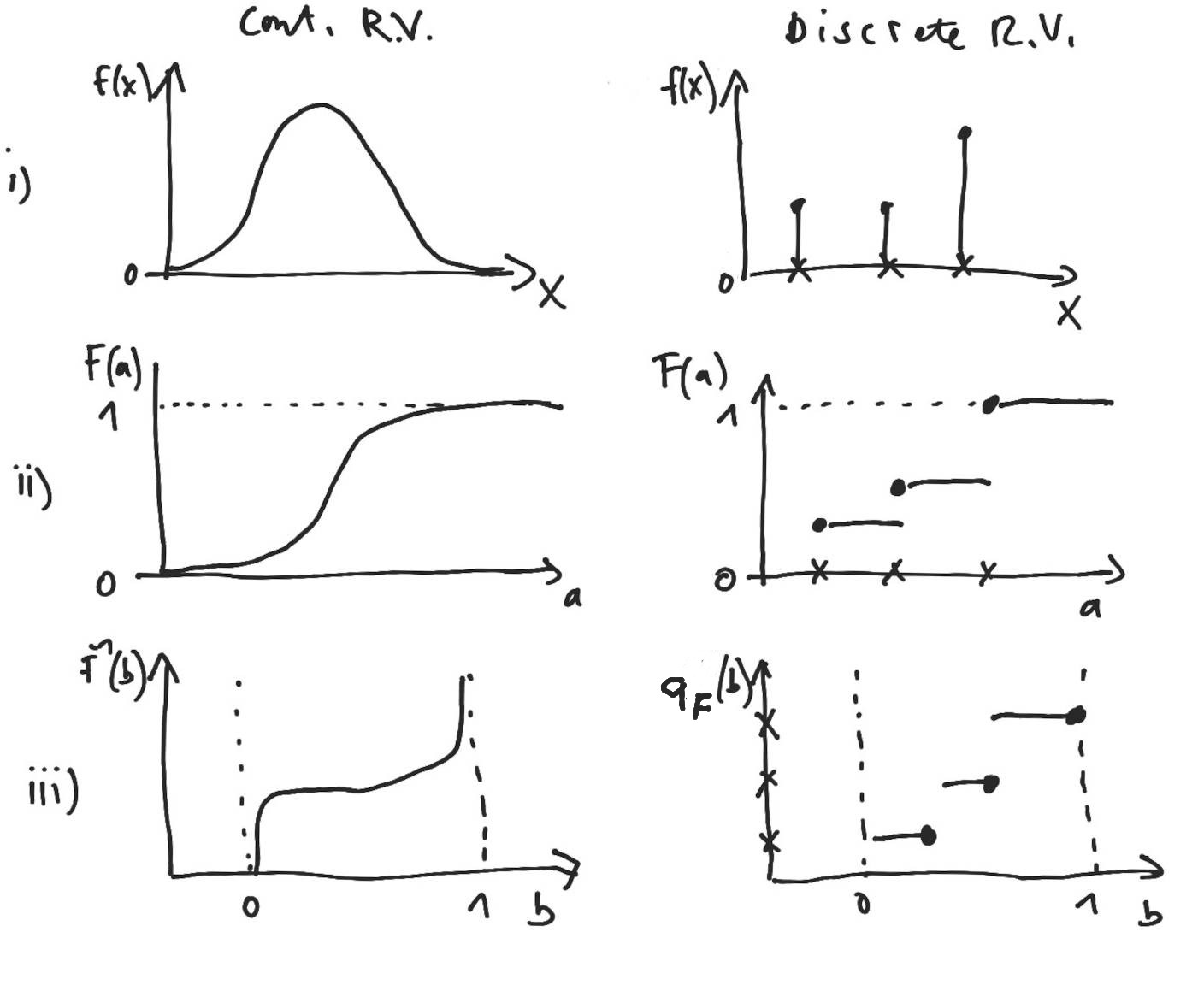
Figure 2.1 (first row) illustrates the pdmf for a continuous and discrete random variable.
In the above we denoted the pdmf by the lower case letter \(f\) though we also often use \(p\) or \(q\).
2.4 Cumulative distribution function
As alternative to the pdmf we can describe the random variable using a cumulative distribution function (cdf). This requires an ordering so that we can define the event \(A = \{x: x \leq a \}\) and compute its probability as \[ F(a) = \operatorname{Pr}(A) = \operatorname{Pr}( x \leq a ) = \begin{cases} \sum_{x \in A} f(x) & \text{discrete case} \\ \int_{x \in A} f(x) dx & \text{continuous case} \\ \end{cases} \] Th cdf is denoted by the same letter as the pdmf but in upper case (usually \(F\), \(P\) and \(Q\)). By construction the cumulative distribution function is monotonically nondecreasing and its value ranges from 0 to 1. For a discrete random variable \(F(a)\) is a step function with jumps of size \(f(\omega_i)\) at the elementary outcomes \(\omega_i\).
With the help of the cdf we can compute the probability of the event \(A = \{x:a_1 < x \leq a_2 \}\) simply as \[ \operatorname{Pr}( A ) = F(a_2)-F(a_1) \,. \] This works both for discrete and continuous random variables.
Figure 2.1 (second row) illustrates the distribution function for a continuous and discrete random variable.
It is common to use the same upper case letter as the cdf to name the distribution. Thus, if a random variable \(x\) has distribution \(F\) we write \(x \sim F\), and this implies it has a pdmf \(f(x)\) and cdf \(F(x)\).
2.5 Quantile function and quantiles
The quantile function is defined as \(q_b(F) = \inf\{ x: F(x) \geq b \}\). For a continuous random variable the quantile function simplifies to \(q_b(F) = F^{-1}(b)\), i.e. it is the ordinary inverse \(F^{-1}(b)\) of the cumulative distribution function.
Figure 2.1 (third row) illustrates the quantile function for a continuous and discrete random variable.
The quantile \(x\) of order \(b\) of the distribution \(F\) is often denoted by \(x_b= q_b(F)\).
The 25% quantile \(x_{1/4} = x_{25\%} = q_{1/4}(F)\) is called the first quartile or lower quartile.
The 50% quantile \(x_{1/2} = x_{50\%} = q_{1/2}(F)=\operatorname{Median}(F)\) is called the second quartile or median.
The 75% quantile \(x_{3/4} = x_{75\%} = q_{3/4}(F)\) is called the third quartile or upper quartile.
The interquartile range is the difference between the upper and lower quartiles and equals \(\operatorname{IQR}(F) = q_{3/4}(F) - q_{1/4}(F)\).
The quantile function is also useful for generating general random variates from uniform random variates. If \(y\sim \operatorname{Unif}(0,1)\) then \(x=q_y(F) \sim F\).
2.6 Expectation or mean
The expected value of a random variable \(x\sim F\) is defined as the weighted average over all possible outcomes, with the weight given by the pdmf \(f(x)\): \[ \begin{split} \operatorname{E}(x) &= \operatorname{E}_F(x) = \operatorname{E}(F)\\ & = \begin{cases} \sum_{x \in \Omega} f(x) \, x & \text{discrete case} \\ \int_{x \in \Omega} f(x) \, x \, dx & \text{continuous case} \\ \end{cases}\\ \end{split} \] The subscript \(F\) in \(\operatorname{E}_{F}(x)\) indicates that the expectation is taken with regard to the distribution \(F\), but is usually left out if there are no ambiguities. The notation \(\operatorname{E}(F)\) emphasises that the mean is a functional of the distribution \(F\).
Because the sum or integral may diverge, not all distributions have finite means so the mean does not always exist (in contrast to the median, or quantiles in general). For example, the location-scale \(t\)-distribution \(t_{\nu}(\mu, \tau^2)\) does not have a mean for a degree of freedom in the range \(0 < \nu \leq 1\) (see Section 5.8).
Expectation is a linear operator, meaning that \[ \operatorname{E}(a_1 x_1 + a_2 x_2) = a_1 \operatorname{E}(x_1) + a_2 \operatorname{E}(x_2) \] for random variables \(x_1\sim F_1\) and \(x_2 \sim F_2\) and constants \(a_1\) and \(a_2\).
Consequently, expectation is mixture preserving so that \[ \operatorname{E}(Q_{\lambda}) = (1-\lambda) \operatorname{E}(Q_0) + \lambda \operatorname{E}(Q_1) \] for the mixture \(Q_{\lambda}=(1-\lambda) Q_0 + \lambda Q_1\) with \(0 < \lambda < 1\) and \(Q_0 \neq Q_1\).
2.7 Variance
The variance of a random variable \(x\sim F\) is the expected value of the squared deviation around the mean \(\mu = \operatorname{E}(x)\): \[ \begin{split} \operatorname{Var}(x) &= \operatorname{Var}_F(x) = \operatorname{Var}(F)\\ &= \operatorname{E}\left( (x - \mu))^2 \right) \\ &= \operatorname{E}(x^2)-\mu^2 \end{split} \] By construction, \(\operatorname{Var}(x) \geq 0\).
The notation \(\operatorname{Var}(F)\) highlights that the variance is a functional of the distribution \(F\). Occasionally, we write \(\operatorname{Var}_F(x)\) indicate that the expectation is taken with regard to the distribution \(F\).
Like the mean, the variance may diverge and hence not necessarily exists for all distribution. For example, the location-scale \(t\)-distribution \(t_{\nu}(\mu, \tau^2)\) does not have a variance for the degree of freedom in the range \(0 < \nu \leq 2\) (see Section 5.8).
2.8 Moments of a distribution
The \(n\)-th moment of a distribution \(F\) for a random variable \(x\) is defined as follows: \[ \mu_n(F) = \operatorname{E}(x^n) \]
Special important cases are the
- Zeroth moment: \(\mu_0(F) = \operatorname{E}(x^0) = 1\) (since the pdmf integrates to one)
- First moment: \(\mu_1(F) = \operatorname{E}(x^1) = \operatorname{E}(x) = \mu\) (=the mean)
- Second moment: \(\mu_2(F) = \operatorname{E}(x^2)\)
The \(n\)-th central moment centred around the mean \(\operatorname{E}(x) = \mu\) is given by \[ m_n(F) = \operatorname{E}((x-\mu)^n) \]
The first few central moments are the
- Zeroth central moment: \(m_0(F) = \operatorname{E}((x-\mu)^0) = 1\)
- First central moment: \(m_1(F) = \operatorname{E}((x-\mu)^1) = 0\)
- Second central moment: \(m_2(F) = \operatorname{E}\left( (x - \mu)^2 \right)\) (=the variance)
The moments of a distribution are not necessarily all finite, i.e. some moments may not exist. For example, the location-scale \(t\)-distribution \(t_{\nu}(\mu, \tau^2)\) only has finite moments of degree smaller than the degree of freedom \(\nu\) (see Section 5.8).
2.9 Expectation of a transformed random variable
Often, one needs to find the mean of a transformed random variable. If \(x\sim F_x\) and \(y= h(x)\) with \(y \sim F_y\) then one can directly apply the above definition to obtain \(\operatorname{E}(y) = \operatorname{E}(F_y)\). However, this requires knowledge of the transformed pdmf \(f_y(y)\) (see Chapter 3 for more details about variable transformations).
As an alternative, the “law of the unconscious statistician”(LOTUS) provides a convenient shortcut to compute the mean of the transformed random variable \(y=h(x)\) using only the pdmf of the original variable \(x\): \[ \operatorname{E}(h(x)) = \begin{cases} \sum_{x \in \Omega} f(x) \, h(x) & \text{discrete case} \\ \int_{x \in \Omega} f(x) \, h(x) \, dx & \text{continuous case} \\ \end{cases} \] Note this is not an approximation but equivalent to obtaining the mean using the transformed pdmf.
2.10 Probability as expectation
Probability itself can also be understood as an expectation.
For an event \(A \subseteq \Omega\) we define a corresponding indicator function \([x \in A]\). From LOTUS it then follows immediately that \[ \begin{split} \operatorname{E}\left( \left[x \in A\right] \right) &= \begin{cases} \sum_{x \in A} f(x) & \text{discrete case} \\ \int_{x \in A} f(x) \, dx & \text{continuous case} \\ \end{cases}\\ & =\operatorname{Pr}(A) \end{split} \]
This relation is called the “fundamental bridge” between probability and expectation. Interestingly, one can develop the whole theory of probability from this perspective (e.g., Whittle 2000).
2.11 Jensen’s inequality for the expectation
If \(h(\boldsymbol x)\) is a convex function then the following inequality holds:
\[ \operatorname{E}(h(\boldsymbol x)) \geq h(\operatorname{E}(\boldsymbol x)) \]
Recall: a convex function (such as \(x^2\)) has the shape of a “valley”.
An example of Jensen’s inequality is \(\operatorname{E}(x^2)\geq \operatorname{E}(x)^2\).
2.12 Random vectors and their mean and variance
In addition to scalar random variables we often make use of random vectors and random matrices.2
The mean of a random vector \(\boldsymbol x= (x_1, x_2,...,x_d)^T \sim F\) is given by \[ \begin{split} \operatorname{E}(\boldsymbol x) &= \operatorname{E}(F) \\ &= \underbrace{\boldsymbol \mu}_{d \times 1} = (\mu_1, \ldots, \mu_d)^T\\ \end{split} \] and thus is a vector of the same dimension as \(\boldsymbol x\), where \(\mu_i = \operatorname{E}(x_i)\) are the means of the individual components \(x_i\).
The variance of a random vector \(\boldsymbol x\) of length \(d\), however, is not a vector but a matrix of size \(d\times d\). This matrix is called the covariance matrix: \[ \begin{split} \operatorname{Var}(\boldsymbol x) &= \operatorname{Var}(F) \\ &= \underbrace{\boldsymbol \Sigma}_{d\times d} = (\sigma_{ij}) = \begin{pmatrix} \sigma_{11} & \dots & \sigma_{1d}\\ \vdots & \ddots & \vdots \\ \sigma_{d1} & \dots & \sigma_{dd} \end{pmatrix} \\ &=\operatorname{E}\left(\underbrace{(\boldsymbol x-\boldsymbol \mu)}_{d\times 1} \underbrace{(\boldsymbol x-\boldsymbol \mu)^T}_{1\times d}\right) \\ & = \operatorname{E}(\boldsymbol x\boldsymbol x^T)-\boldsymbol \mu\boldsymbol \mu^T \\ \end{split} \] The elements \(\operatorname{Cov}(x_i, x_j)=\sigma_{ij}\) describe the covariance between the random variables \(x_i\) and \(x_j\). The covariance matrix is symmetric, hence \(\sigma_{ij}=\sigma_{ji}\). The diagonal elements \(\operatorname{Cov}(x_i, x_i)=\sigma_{ii}\) correspond to the individual variances \(\operatorname{Var}(x_i) = \sigma_i^2\). By construction, the covariance matrix \(\boldsymbol \Sigma\) is positive semidefinite, i.e. the eigenvalues of \(\boldsymbol \Sigma\) are all positive or equal to zero.
However, wherever possible one will aim to use models with nonsingular covariance matrices, with all eigenvalues positive, so that the covariance matrix is invertible.
2.13 Correlation matrix
The correlation matrix \(\boldsymbol P\) (“upper case rho”, not “upper case p”) is the variance standardised version of the covariance matrix \(\boldsymbol \Sigma\).
Specifically, denote by \(\boldsymbol V\) the diagonal matrix containing the variances \[ \boldsymbol V= \begin{pmatrix} \sigma_{11} & \dots & 0\\ \vdots & \ddots & \vdots \\ 0 & \dots & \sigma_{dd} \end{pmatrix} \] then the correlation matrix \(\boldsymbol P\) is given by \[ \boldsymbol P= (\rho_{ij}) = \begin{pmatrix} 1 & \dots & \rho_{1d}\\ \vdots & \ddots & \vdots \\ \rho_{d1} & \dots & 1 \end{pmatrix} = \boldsymbol V^{-1/2} \, \boldsymbol \Sigma\, \boldsymbol V^{-1/2} \] Like the covariance matrix the correlation matrix is symmetric. The elements of the diagonal of \(\boldsymbol P\) are all set to 1.
Equivalently, in component notation the correlation between \(x_i\) and \(x_j\) is given by \[ \rho_{ij} = \operatorname{Cor}(x_i,x_j) = \frac{\sigma_{ij}}{\sqrt{\sigma_{ii}\sigma_{jj}}} \]
Following from the definition above, a covariance matrix \(\boldsymbol \Sigma\) can be factorised into the product of standard deviations \(\boldsymbol V^{1/2}\) and the correlation matrix \(\boldsymbol P\) as follows: \[ \boldsymbol \Sigma= \boldsymbol V^{1/2}\, \boldsymbol P\,\boldsymbol V^{1/2} \]
2.14 Parameters and families of distributions
A distribution family \(F(\theta)\) is a collection of distributions obtained by varying a parameter \(\theta\). Each specific value of the parameter \(\theta\) indexes one distribution in that family.
Common distribution families are usually denoted by familiar abbreviation such as \(N(\mu, \sigma^2)\) for the normal family. We also call these simply “distributions” with parameters and omit the word “family”.
If a random variable \(x\) has distribution \(F(\theta)\) we write \(x \sim F(\theta)\). In case of named distributions, we use the corresponding abbreviation such \(x \sim N(\mu, \sigma^2)\) (normal distribution) or \(x \sim \operatorname{Beta}(\alpha_1, \alpha_2)\).
The associated pdmf is written \(f(x; \theta)\) or \(f(x | \theta)\). The conditional notation is more general because it implies the parameter \(\theta\) may have its own distribution, yielding a joint density \(f(x, \theta) = f(x | \theta) f(\theta)\). Similarly, the corresponding cumulative distribution function is written \(F(x; \theta)\) or \(F(x | \theta)\).
Note that parametrisations are generally not unique, as any one-to-one transformation of \(\theta\) yields an equivalent index of the same distribution family. For most commonly used distribution families there exist several standard parametrisations. We usually prefer those whose parameters that can be interpreted easily (e.g. in terms of moments) or that help to simplify calculations.
If distinct parameters correspond to distinct distributions, they are called identifiable. This is an important property as it allows parameters to be estimated from data. Specifically, if parameters are identifiable then \(P(\theta_1) = P(\theta_2)\) implies \(\theta_1 = \theta_2\), and conversely if \(P(\theta_1) \neq P(\theta_2)\) then \(\theta_1 \neq \theta_2\). If parameters and distributions are unique within a neighbourhood \(\theta_0+\epsilon\) relative to a reference value \(\theta_0\), rather than globally, they are locally identifiable at \(\theta_0\).
The dimension of a distribution family equals the dimension of its parameter space and is the number of parameters in a minimal parametrisation. This is not to be confused with the dimension of the random variable (i.e. univariate or multivariate).
An important class of distribution families are exponential families discussed in Chapter 7.
This notation is common in statistical machine learning and multivariate statistics, see for example Mardia et al. (1979). An alternative convention uses uppercase letters for random variables and lowercase for outcomes, but that convention is problematic for multivariate objects (random vectors and random matrices) and is also ill-suited in Bayesian statistics where parameters are modelled as random variables.↩︎
In our notational conventions, a scalar \(x\) is written in lower case plain font, a vector \(\boldsymbol x\) is written in lower case bold font, a matrix \(\boldsymbol X\) in upper case bold font.↩︎